What is sound, movement, vibration, sensation? - Signal Processing for Interactive Systems

from IPython.display import display, YouTubeVideo, Image

Sound is a vibration which travels through a medium as

longitudinal waves: gasses (e.g., air), liquids (e.g., water), and solids (e.g., concrete)
transversal sound waves: solids (e.g., concrete)

The speed of sound depends on the medium.

In air at room temperature, for example, it is approximately 343 m/s.

Image('apLecture1_files/wave.png')

Sound is normally divided into three types:

Infrasound: Sound with frequencies up to 20 Hz
Audible sound: Sound with frequencies in range 20 Hz - 20 kHz (audio)
Ultrasound: Sound with frequencies above 20 kHz

We can consider haptics as slow vibrations too.

Human hearing¶

The human ear consists of the following parts:

Outer ear: Everything on the outside of the ear drum, including the pinna
Middle ear: The three bones (Malleus, Incus, Stapes). What do they do?
Inner ear: The cochlea (Latin for what?) tube. What does the basilar membrane do inside? Hair cells?

The human ear

does not hear all frequencies equally well
is most sensitive to frequencies around 4 kHz
is tuned to speech
has a really large dynamic range of up to ~120 dB (i.e., we can hear sound intensities up to ~10^12 the quietest sounds)

Human ear

Sinusoids¶

A sinusoid (or a sine wave) is given by

x(t) = A \cos(\Omega t + \Phi)

(1)

where

$A\geq0$ is the amplitude
$\Omega$ is the frequency measured in radians pr. second (SI symbol rad/s). Is related to the frequency $f$ measured in cycles pr. second (SI symbol Hz) via $\Omega = 2\pi f$ .
$t$ is the time measured in seconds (SI symbol s)
$\Phi$ is the initial phase measured in radians (SI symbol rad)

The above form of the sinusoid is often referred to as the polar form. By using the angle addition formula for a cosine, i.e.,

\cos(\theta+\phi) = \cos(\theta)\cos(\phi)-\sin(\theta)\sin(\phi)\ ,

(2)

a sinusoid can also be written in a rectangular form as

x(t) = a\cos(\Omega t) + b\sin(\Omega t)

(3)

where a and b are scalars given by

\begin{align} a &= A\cos(\Phi)\\ b &= -A\sin(\Phi)\ . \end{align}

(4)

Numpy example: A sinusoid¶

%matplotlib inline
import numpy as np
import matplotlib.pyplot as plt

samplingFreq = 44100 # Hz
nData = 2000
time = np.arange(0,nData).T/samplingFreq # s

# Generate a sinusoid
amp = 1;
freq = 100 # Hz
initPhase = np.pi/2 # rad
sinusoid = amp*np.cos(2*np.pi*freq*time+initPhase)
 
# Plot the sinusoids
plt.plot(time, sinusoid, linewidth=2)
plt.xlim((time[0],time[nData-1]))
plt.ylim((-1,1))
plt.xlabel('Time [s]')
plt.ylabel('Amplitude [.]')
plt.grid(True)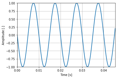

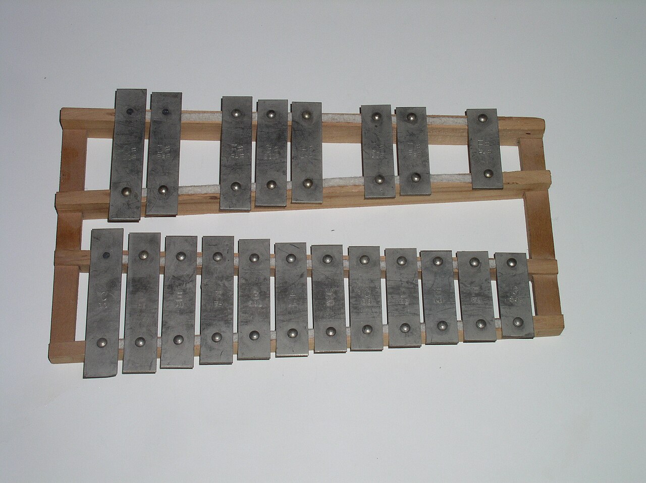
Example: Generation of a sinusoid from a vibrating bar (Newton to Nada Brahma)¶

Glockenspiel

Assume that the act of striking a bar is modelled as compressing a spring in one dimension.

From Hooke’s law, this compresssion can be written as

F(t) = -k x(t)

(5)

where

$F(t)$ is the restoring force measured in Newton (SI unit N)
$x(t)$ is the displacement measured in meters (SI unit m) of the string from its resting position
$k$ is the spring constant measured in N/m

From Newton’s second law, the force can also be expressed as

F(t) = ma(t)

(6)

where

$m$ is the mass of the string measured in kilogram (SI unit kg)
$a(t)$ is the acceleration measured in m/s^2.

The acceleration is related to the displacement $x(t)$ as

a(t) = \frac{dv(t)}{dt} = \frac{d^2 x(t)}{d t^2}

(7)

where $v(t)$ is the velocity measured in m/s.

Combining these three equations gives

-k x(t) = F(t) = ma(t) = m \frac{d^2 x(t)}{dt^2}

(8)

which can be rewritten as

\frac{d^2 x(t)}{dt^2} = -\frac{k}{m} x(t)\ .

(9)

This is a constant-coefficient second-order differential equation.

Let us check if our sinusoid

x(t) = A\cos(\Omega t + \Phi)

(10)

is a solution to the above differential equation. Since

\begin{align} \frac{dx(t)}{dt} &= -\Omega A\sin(\Omega t + \Phi)\\ \frac{d^2 x(t)}{d t^2} &= -\Omega^2 A\cos(\Omega t + \Phi) = -\Omega^2 x(t)\ , \end{align}

(11)

we obtain

-\Omega^2x(t) = -\frac{k}{m} x(t)\ .

(12)

Thus, striking a bar will make it vibrate sinusoidally with the frequency

\Omega = \sqrt{k/m}\ .

(13)

This frequency can be changed by changing the spring constant and mass.

Summary¶

Sound is a vibration travelling through a medium.
Sound waves are longitudal waves (and also transversal waves when travelling through a solid).
The human ear converts pressure variations in the air to

mechanical movement (interface is the eardrum)
vibrations in a liquid (interface is the oval window)
electrical signal to the brain (interface is the haircells attached to the basilar membrane)

A sinusoid (or sine wave) is given by
$x(t) = A\cos(\Omega t + \Phi)\ ,$
(14)
and it an extremely important building block (or atom) in analysing and manipulating sound.
Assuming that striking a bar can be modelled as compressing a spring, the bar will vibrate sinusoidally.

Complex numbers¶

In the next 20 minutes, you will learn

that the equation
$x^2+1=0$
(15)
has two solutions
what a complex number is
how you add and multiply complex numbers

The need for complex numbers¶

While the linear equation

x + 1 = 0

(16)

can easily be solved, the simple quadratic equation

x^2 + 1 = 0

(17)

was in high school said to have no solution since its descriminant was negative.

%matplotlib inline
import numpy as np
import matplotlib.pyplot as plt

nData = 100
x = np.linspace(-2,2,nData)
y = x**2+1
plt.plot(x,y,linewidth=2)
plt.xlabel('x')
plt.ylabel('y')
plt.ylim((-1,5))
plt.grid(True);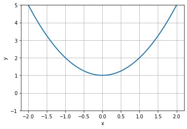

However, the quadratic equation can in fact be solved by using complex numbers.

Rearranging our simple quadratic equation gives

x^2 = -1

(18)

which allows us to write the solution as

x = \pm\sqrt{-1} = \pm j

(19)

where

j = \sqrt{-1}

(20)

is the imaginary unit. This unit also satisfies that

j^2 = \sqrt{-1}^2 = -1\ .

(21)

Note that

engineers normally use the symbol $j$ for the imaginary unit
mathematicians normally use the symbol $i$ for the imaginary unit.

Let us now consider the quadratic equation

x^2 + 2x + 5 = 0\ .

(22)

We know from high school that the solutions to the general quadratic

ax^2 + bx + c = 0\ ,\qquad\text{for }a\neq0

(23)

have the form

x = \frac{-b\pm\sqrt{d}}{2a}

(24)

where $d$ is the discriminant given by

d = b^2-4ac\ .

(25)

We obtain

d = 4-20 = -16

(26)

so that

x = \frac{-2\pm\sqrt{-16}}{2} = -1\pm\frac{1}{2}\sqrt{-1\cdot 4^2} = -1\pm 2\sqrt{-1} = -1\pm 2j\ .

(27)

Thus, the complex numbers $-1+2j$ and $-1-2j$ are the solutions.

The complex number¶

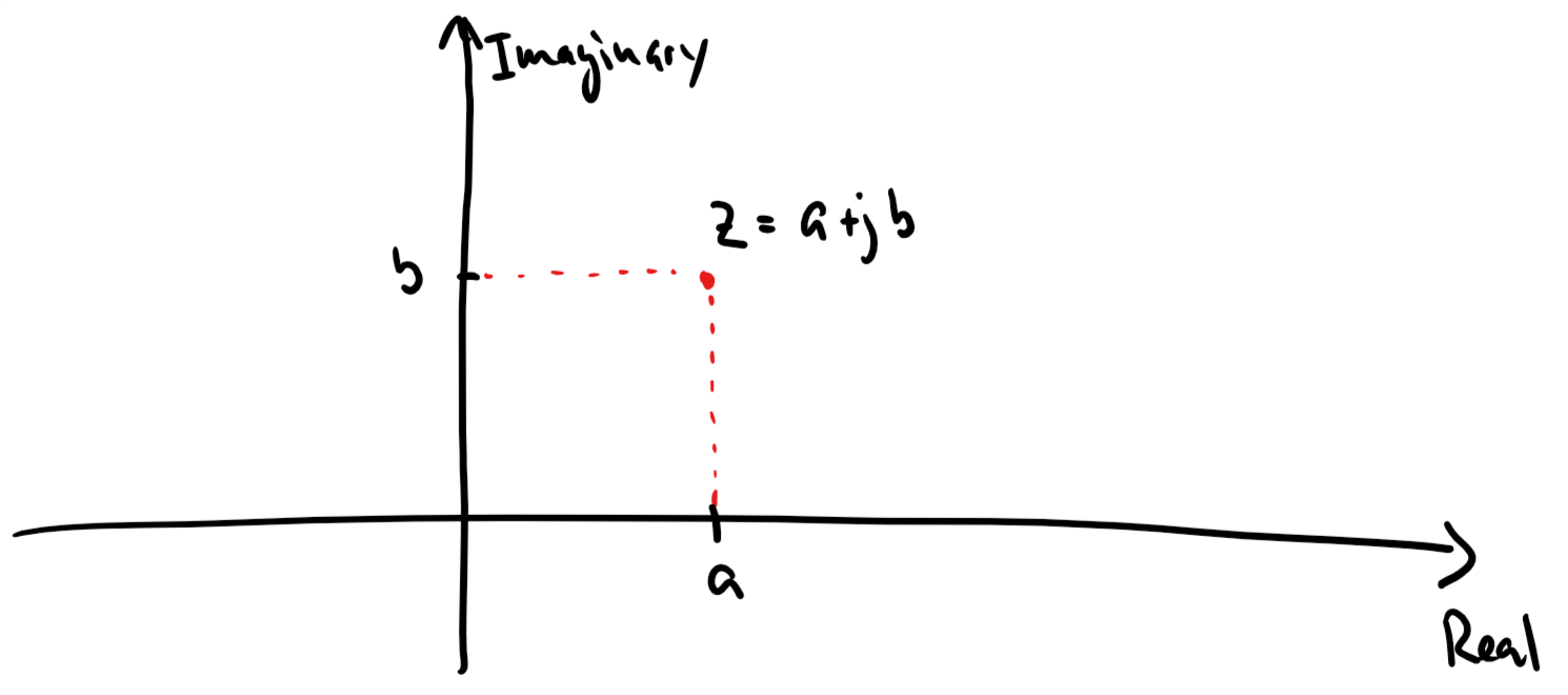
A complex number can be written as

z = a + jb

(28)

where

$a = \text{Re}\{z\}$ is the real part
$b = \text{Im}\{z\}$ is the imaginary part.

A complex number can be depicted in the complex plane which is a 2D coordinate system.

Complex plane

The complex conjugate¶

The complex conjugate of a complex number $z$ is

z^* = a - jb\ .

(29)

Thus, the conjugation operator ${}^*$ changes the sign of imaginary part, but not the real part.

Addition of complex numbers¶

Assume we have the two complex numbers

\begin{align} z_1 &= a_1+jb_1\\ z_2 &= a_2+jb_2\ . \end{align}

(30)

The sum of these two numbers is then

z = z_1 + z_2 = a_1+jb_1 + a_2+jb_2 = (a_1+a_2) + j(b_1+b_2).

(31)

Thus, the real and imaginary part of of $z=a+jb$ are simply

\begin{align} a &= a_1 + a_2\\ b &= b_1 + b_2\ . \end{align}

(32)

Note that

\begin{align} z_1 + z_1^* &= 2a_1 + 0j = 2\text{Re}(z_1)\\ z_1 - z_1^* &= 0 + 2jb_1 = 2\text{Im}(z_1)\ . \end{align}

(33)

Multiplication of complex numbers¶

Assume we have the two complex numbers

\begin{align} z_1 &= a_1+jb_1\\ z_2 &= a_2+jb_2\ . \end{align}

(34)

The product of these two numbers is then

z = z_1z_2 = (a_1+jb_1)(a_2+jb_2) = (a_1a_2-b_1b_2) + j(a_1b_2+b_1a_2).

(35)

Thus, the real and imaginary part of of $z=a+jb$ are

\begin{align} a &= (a_1a_2-b_1b_2)\\ b &= (a_1b_2+b_1a_2)\ . \end{align}

(36)

Note that

z_1z_1^* = (a_1a_1-b_1(-b_1)) +j(a_1b_1-b_1a_1) = a_1^2+b_1^2 = \text{Re}(z_1)^2+\text{Im}(z_1)^2

(37)

Summary¶

Complex numbers were originally invented to solve algebraic equations (e.g., the cubic equation)
The imaginary unit is $j=\sqrt{-1}$
A complex number $z$ consists of a real part $a$ and imaginary part $b$ , and is written as
$z = a+jb\ .$
(38)
The complex conjugate of $z$ is
$z^* = a-jb\ .$
(39)
It is much easier to add two complex numbers than it is to multiply them.

Additional information on complex numbers¶

If you want to know more about complex numbers, you can find some nice videos here:

Exit Question¶

Let

\begin{align} z_1 &= a_1+jb_1 = 2+3j\\ z_2 &= a_2+jb_2 = -1-2j\ . \end{align}

(40)

By hand, please calculate

\begin{align} z_1 + z_2 &= \\ z_1 - z_2 &= \\ z_1 + z_1^* &= \\ z_2 - z_2^*+2z_1 &= \\ z_1z_2^* &=\\ z_1^2+z_2^*z_1 &= \end{align}

(41)

Check the results with your neighbours.

Tip: Use the rules

\begin{align} z_1 + z_2 &= (a_1+a_2) + j(b_1+b_2)\\ z_1z_2 &= (a_1a_2-b_1b_2) + j(a_1b_2+b_1a_2)\ . \end{align}

(42)

Phasors¶

In the next 20 minutes, you will learn

how a complex number can be written in a polar form
why the polar form makes multiplications much easier
what a phasor is
how a phasor is related to a real sinusoid

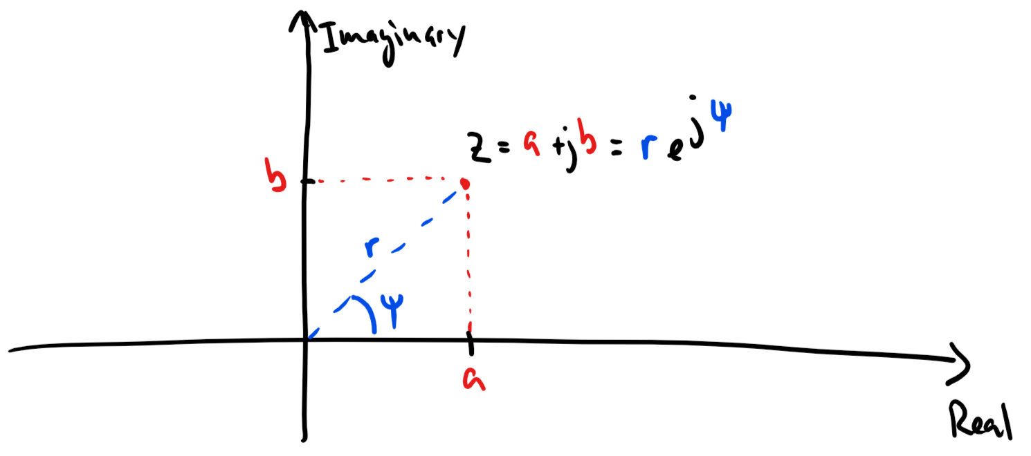
The polar (or exponential) form of a complex number¶

As for 2D vectors, we can also write a complex number in terms of its magnitude $r$ and angle $\psi$ . We have

\begin{align} a &= r\cos\psi\\ b &= r\sin\psi\ . \end{align}

(43)

Thus,

z = a + jb = r\left(\cos\psi + j\sin\psi\right) = r\mathrm{e}^{j\psi}

(44)

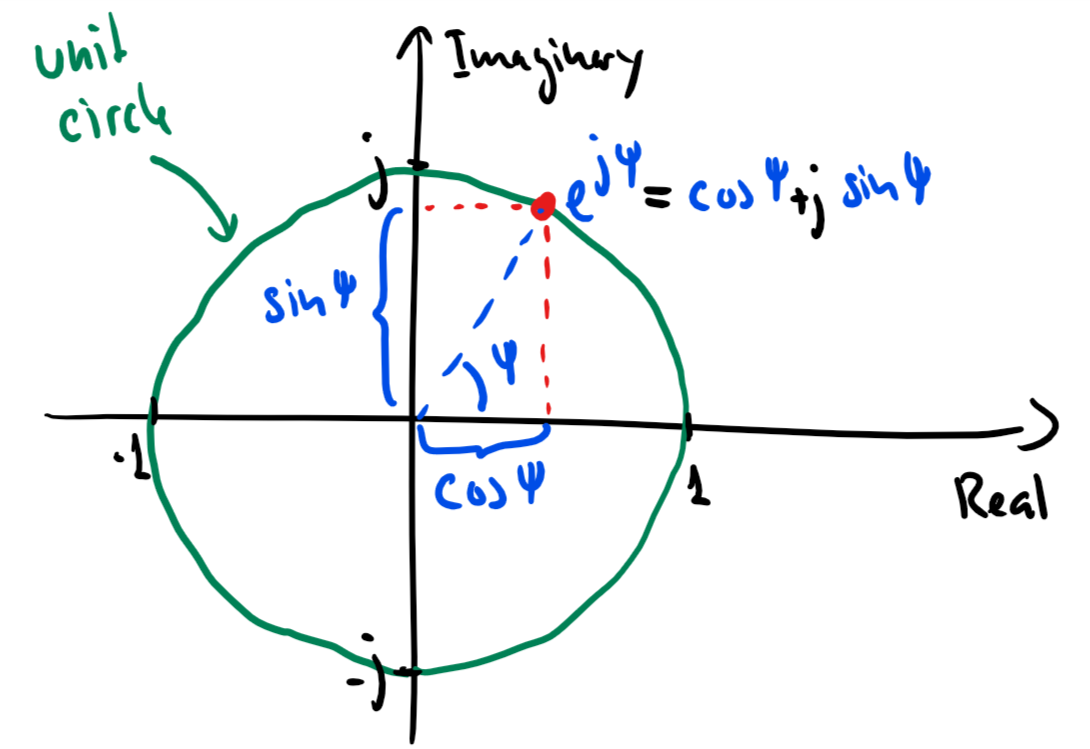
where the last equality follows from Euler’s formula.

Complex plane

Euler’s formula¶

Given by

\mathrm{e}^{j\psi} = \cos\psi + j\sin\psi\ .

(45)

A very important formula used everywhere in science and engineering
Simplifies notation and mathematical manipulations
Its real and imaginary parts are a cosine and a sine, respectively, i.e.,

\begin{align} \text{Re}(\mathrm{e}^{j\psi}) &= \cos\psi\\ \text{Im}(\mathrm{e}^{j\psi}) &= \sin\psi\ . \end{align}

(46)

Complex plane

The complex conjugate¶

The complex conjugate of a complex number

z=r \mathrm{e}^{j\psi}

(47)

is

z^* = r \mathrm{e}^{-j\psi}\ .

(48)

Thus, the conjugation operator ${}^*$ changes the sign of the angle, but not the magnitude.

Multiplication of complex numbers¶

Multiplication of complex numbers is much easier when the polar form is used. Let

\begin{align} z_1 &= a_1+jb_1 = r_1 \mathrm{e}^{j\psi_1}\\ z_2 &= a_2+jb_2 = r_2 \mathrm{e}^{j\psi_2}\ . \end{align}

(49)

The product of these two numbers is then

z = z_1z_2 = r_1 \mathrm{e}^{j\psi_1}r_2 \mathrm{e}^{j\psi_2} = r_1 r_2 \mathrm{e}^{j\psi_1}r_2 \mathrm{e}^{j\psi_2} = r_1 r_2 \mathrm{e}^{j(\psi_1+\psi_2)}

(50)

where we used $a^na^m = a^{n+m}$ to get the last equation.

Thus, to multiply two complex numbers we

multiply their magnitudes
add their angles

Note that divisions can be calculated as multiplications since

\frac{z_1}{z_2} = z_1\frac{1}{z_2} = z_1 z_2^{-1}

(51)

and

z_2^{-1} = \frac{1}{r_2}\mathrm{e}^{-j\psi_2}\ .

(52)

Converting between the rectangular and polar forms¶

We have seen that a complex number $z$ can be written as

z = a+jb = r\mathrm{e}^{j\psi}\ .

(53)

We can convert from the polar coordinates $(r,\psi)$ to the rectangular coordinates $(a,b)$ via

\begin{align} a &= r\cos\psi\\ b &= r\sin\psi\ . \end{align}

(54)

We can convert from the rectangular coordinates $(a,b)$ to the polar coordinates $(r,\psi)$ via

\begin{align} r &= \sqrt{a^2+b^2}\\ \psi &= \mathrm{arctan2}(b,a)\ . \end{align}

(55)

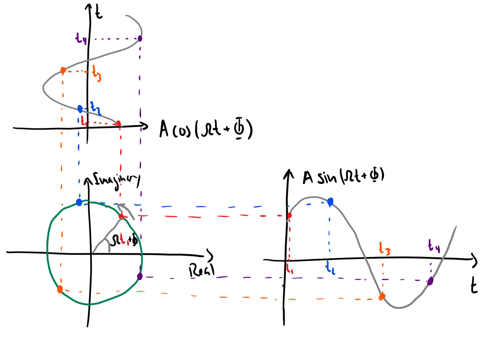
The phasor¶

We have previously looked at the sinusoid

x(t) = A\cos(\Omega t + \Phi)\ .

(56)

Based on what we know about Euler’s formula and complex numbers, we can now also write $x(t)$ as

x(t) = \text{Re}\left[A\exp(j(\Omega t +\Psi))\right]

(57)

since (from Euler’s formula)

A\exp(j(\Omega t +\Psi)) = A\cos(\Omega t +\Psi)+jA\sin(\Omega t +\Psi)\ .

(58)

This time-varying complex number is called a phasor or a complex sinusoid.

Note that

using the phasor instead of the real sinusoid makes life much easier (you will see this later in the course)
even though we work with the phasor, we can always come back to the real sinusoid by taking the real part of the phasor

Phasor illustration

Animated phasors

Summary¶

The polar form of a complex number $z=a+jb$ is
$z = r\mathrm{e}^{j\psi}$
(59)
where the magnitude $r$ and angle $\psi$ are given by

\begin{align} r &= \sqrt{a^2+b^2}\\ \psi &= \mathrm{arctan2}(b,a)\ . \end{align}

(60)

Multiplications (and divisions) are much easier when using the polar form.
A phasor is a complex sinusoid given by
$z(t) = A\exp(j(\Omega t +\Psi))\ ,$
(61)
and its real part is a real sinusoid, i.e.,
$x(t) = \text{Re}(z(t)) = A\cos(\Omega t +\Psi)\ .$
(62)