Central question

How are analog signals turned into digital representation (i.e., data) on a computer?
How can we analyse these digital signals (i.e. extract information from them)?
How can we modify these signals? How can we convert them back to analog signals?

Sampling and reconstruction¶

In the next 20 minutes, you will learn

What a continuous-time signal is.
What a discrete-time signal is.
How you turn a continuous-time signal into a discrete-time signal (i.e., sampling).
How you turn a discrete-time signal into a continuous-time signal (i.e., reconstruction).

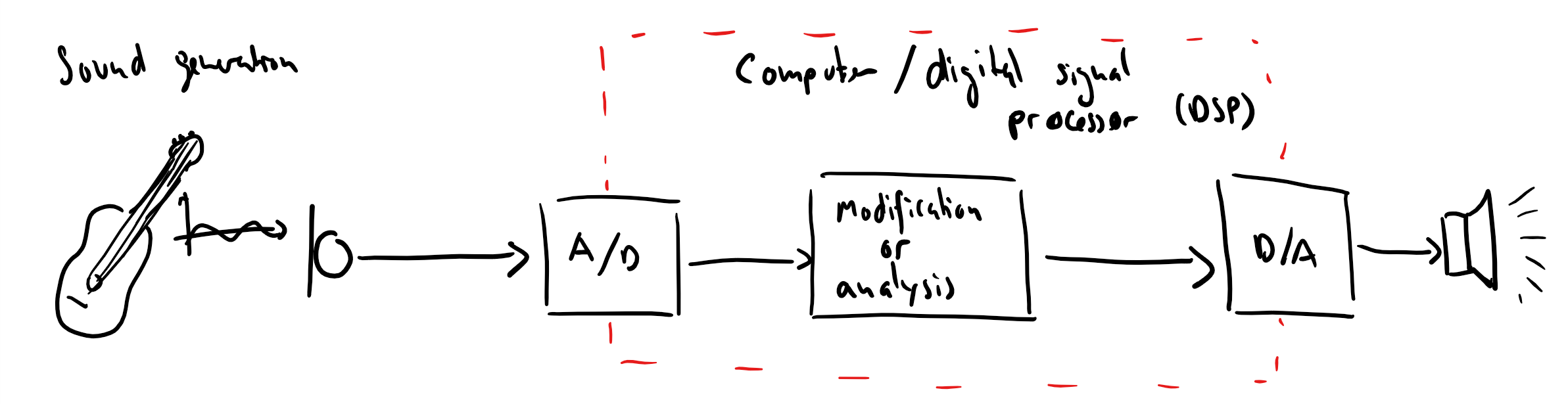
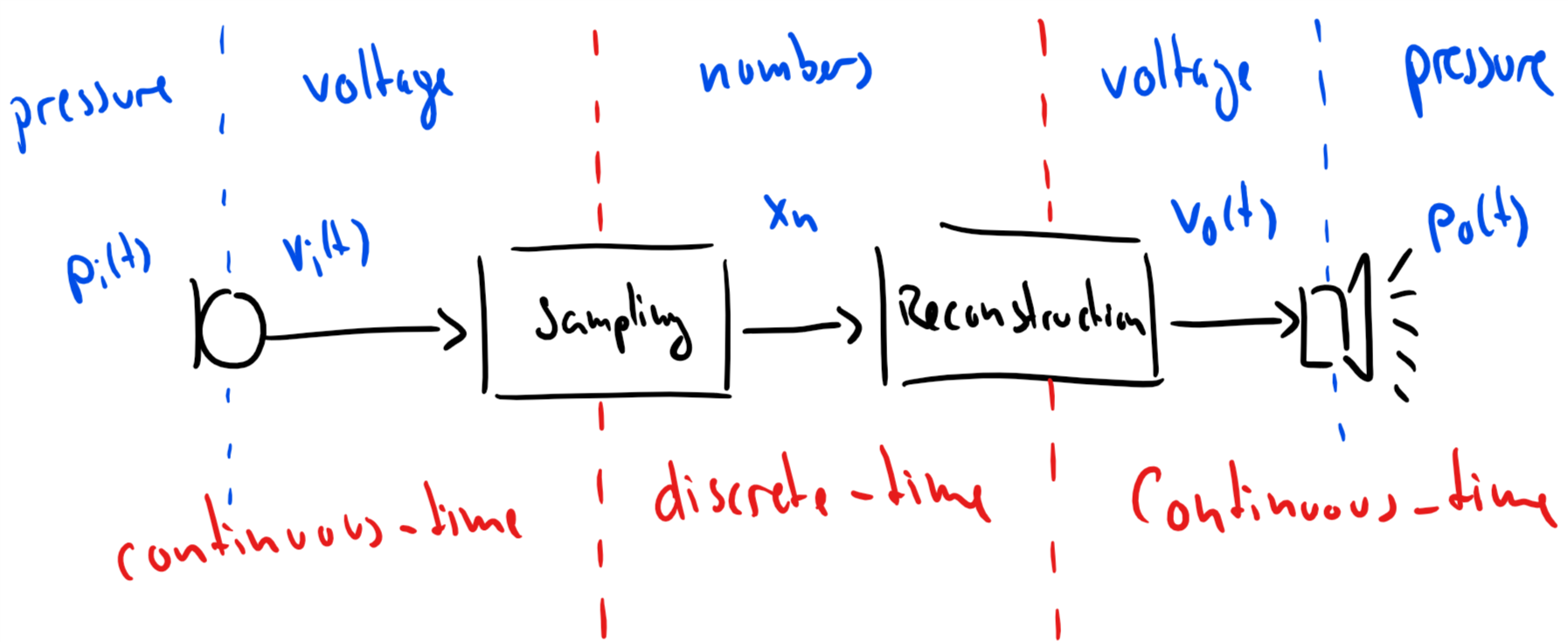
In the figure below, the following is happening:

An audio signal $p_\text{i}(t)$ is propagating through the air as pressure variations.
The microphone picks up the pressure variations and turns them into voltage variations $v_\text{i}(t)$ .
The voltage is converted into a series of numbers $x_n$ via sampling.
A voltage signal $v_\text{o}(t)$ is reconstructed from the series of numbers $x_n$ .
A loudspeaker converts the voltage variations into pressure variations $p_\text{o}(t)$ .

Illustration of sampling and reconstruction

Continuous-time signal¶

A continuous-time signal is characterised by

time: the signal has a value $x(t)$ for every possible time $t$
amplitude: the signal value $x(t)$ can take on any value from a continuum of numbers (such as the real numbers).

A continuous-time signal is often also referred to as an analog signal.

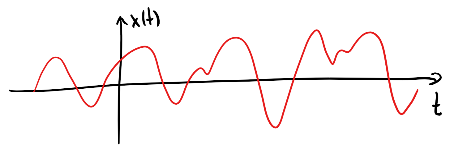
Informally: You draw a continuous-time signal without lifting your pen from the paper.

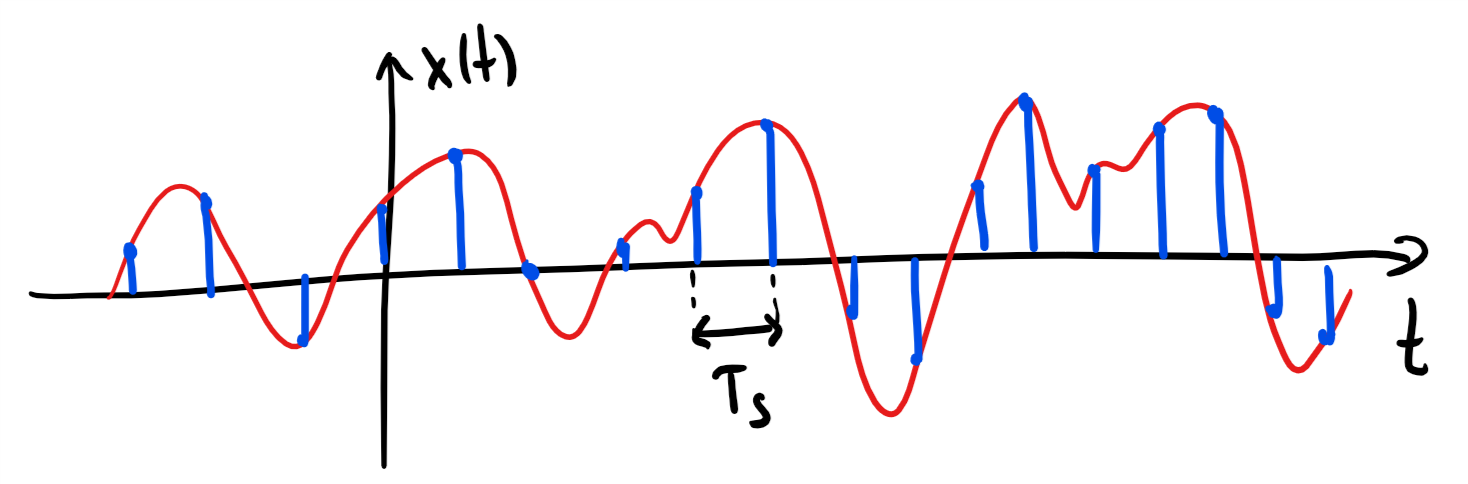
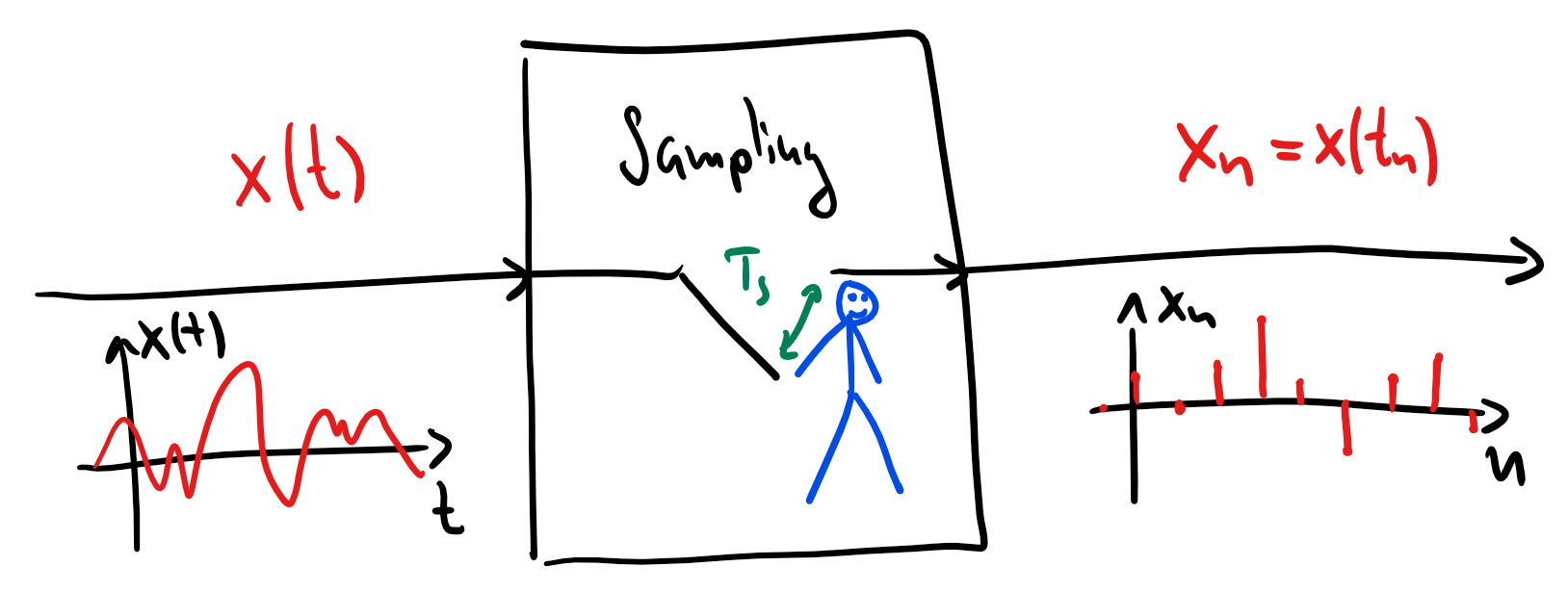
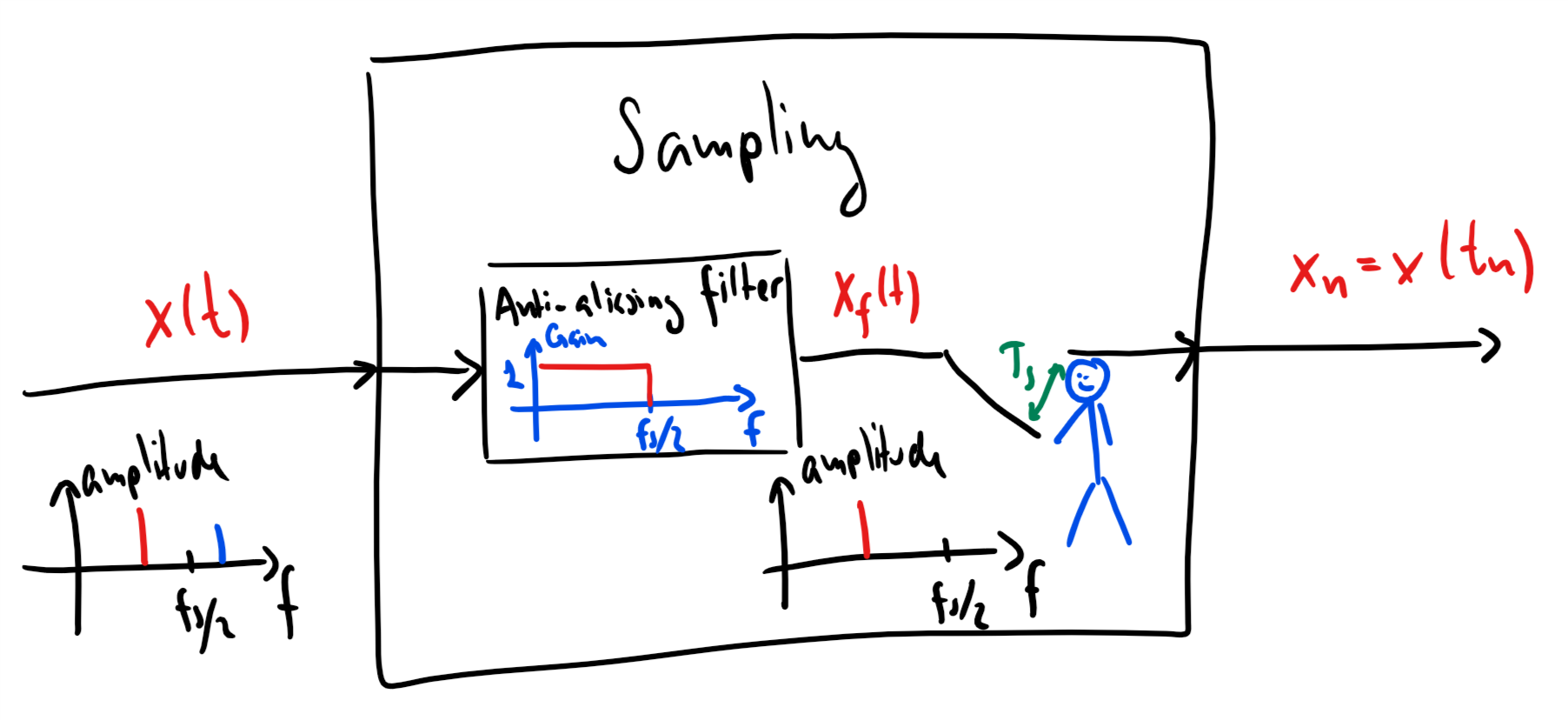
Sampling¶

Storing a continuous-time signal on a computer requires an infinite amount of memory!
Solution: We only measure the value of a continuous-time signal every $T_\text{s}$ seconds. This is called sampling.
A very important quantity is
$f_\text{s} = 1/T_\text{s}$
(1)
where
- $f_\text{s}$ is the sampling frequency (measured in Hz) and describes how many times per second the continuous-time signal is sampled
- $T_\text{s}$ is the sampling time (measured in seconds).

We can illustrate sampling by a person controlling a contact (see figure below):

When $T_\text{s}$ seconds has passed, the contact is pushed and released immidiately.
At that exact time instant, the value of the continuous-time signal $x(T_\text{s})$ is stored on the computer.
After another $T_\text{s}$ seconds, the contact is again pushed and released immidiately so that $x(2T_\text{s})$ is now stored.
If we keep pushing/relasing the contact every $T_\text{s}$ seconds, we will after $n$ times store the signal value $x(t_n)$ where
$t_n = nT_\text{s} = n/f_\text{s}\ .$
(2)
The scaler $n$ is often referred to as the sampling index.

Note that people often write $x(t_n)$ as

x(t_n) = x_n = x[n]\ .

(3)

Discrete-time signal¶

A discrete-time signal is characterised by

time: the signal only has a value $x_n$ at certain times, i.e., $t_n=nT_\text{s}$ for $n=\cdots,-3,-2,1,0,1,2,3,\cdots$ . Therefore, the $x$ -axis is often the sampling index $n$ instead of time.
amplitude: the signal value $x_n$ can take on any value from a continuum of numbers (such as the real numbers).

A discrete-time signal is sometimes also referred to as a digital signal (although we will use this term for something slightly different later).

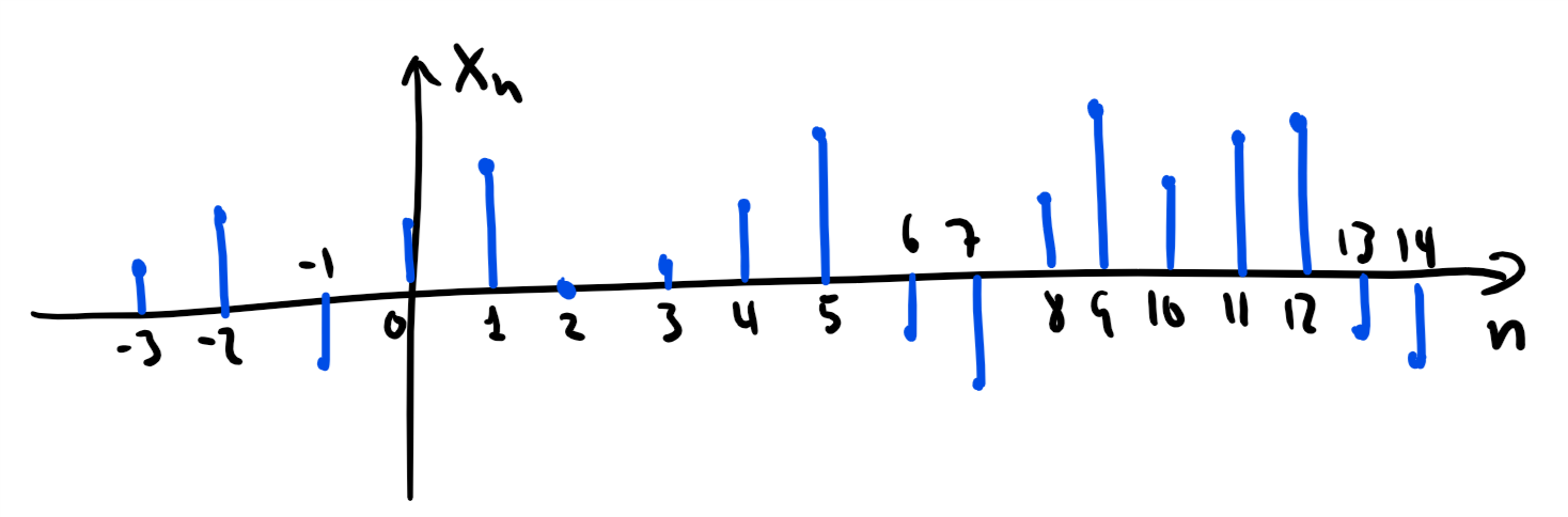
Informally: A discrete-time signal is a series of time-ordered numbers.

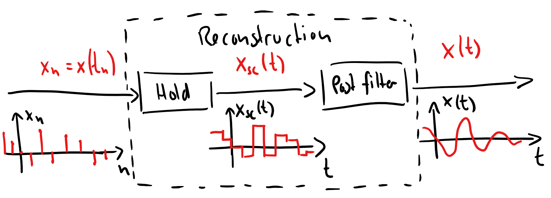
Reconstruction¶

If we want to play back a discrete-time signal on, e.g., a loudspeaker, we have to convert the discrete-time signal back into a continuous-time signal.

Converting a discrete-time signal $x_n$ into a continuous-time signal $x(t)$ is called reconstruction.
Reconstruction is performed using two components:
hold circuit: holds a value $x_n$ for $T_\text{s}$ seconds. This will create a staircase signal.
post filter: smooth out the discountinuities in the staircase signal by using a low-pass filter with a cut-off frequency of $f_\text{s}/2$ Hz.

Note that we will talk much more about filtering in the next lectures.

Summary¶

A continuous-time signal $x(t)$ can be drawn without lifting the pen from the paper.
A discrete-time signal $x_n = x(t_n)$ is a series of time-ordered numbers.
Sampling converts a $x(t)$ into $x_n$ by measuring the value of $x(t)$ at the times
$t_n = nT_\text{s} = n/f_\text{s}$
(4)
where

$n$ is the sampling index
$T_\text{s}$ is the sampling time
$f_\text{s}=1/T_\text{s}$ is the sampling frequency

Reconstruction converts $x_n$ into $x(t)$ by first creating a staircase signal from $x_n$ and then by filtering this staircase signal with a low-pass filter.

Aliasing¶

In the next 20 minutes, you will learn

How we write a discrete-time sinusoid.
What aliasing is.
How we can avoid aliasing by selecting the sampling frequency $f_\text{s}$ .
What an anti-aliasing filter is and why we need it.

Discrete-time sinusoid¶

As we have seen in the first two lectures, a continuous-time sinusoid can be written as

x(t) = A\cos(\Omega t+\psi)

(6)

where

$A\geq 0$ is an amplitude
$\Omega=2\pi f$ is a frequency measured in rad/s
$\psi$ is the inial phase.

Let us now sample this signal with a sampling frequency of $f_\text{s}$ Hz. We then get the discrete-time sinusoid

\begin{align} x_n &= x(t_n) = x(n/f_\text{s}) = A\cos(\Omega n/f_\text{s}+\psi) = A\cos((2\pi f/f_\text{s}) n+\psi)\\ &= A\cos(\omega n+\psi) \end{align}

(7)

where

$\omega = \Omega f_\text{s}= 2\pi f/f_\text{s}$ is the digital frequency measured in radians/sample.

For a discrete-time signal, $\omega = 2\pi$ corresponds to the sampling frequency, and we will also write this frequency as $\omega_\text{s}$ .

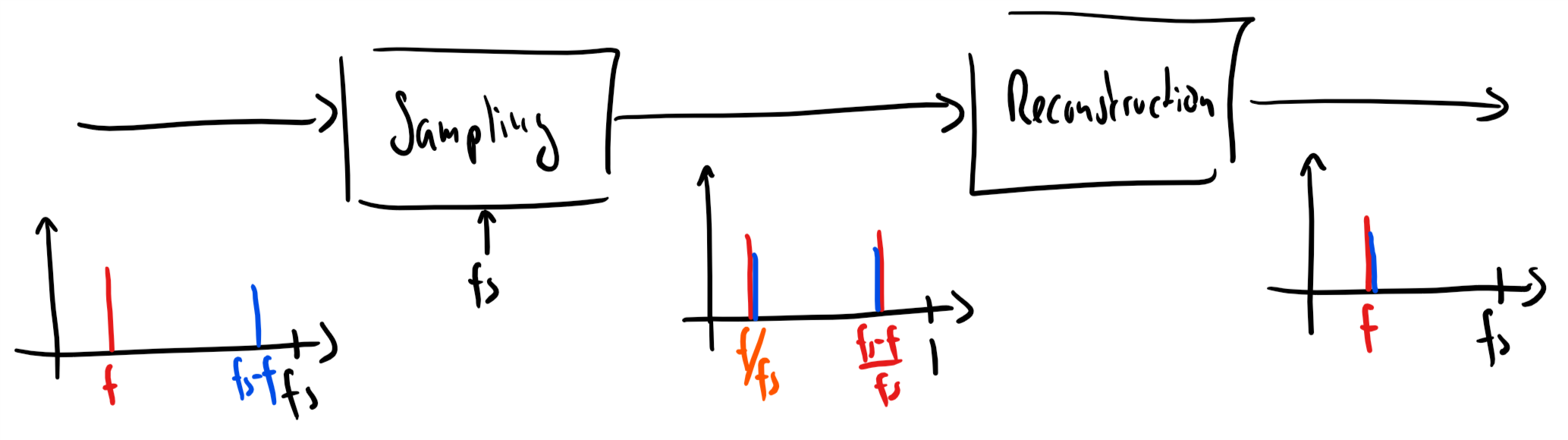
What is Aliasing?¶

Aliasing comes from the word alias.
It refers to that a sinusoidal component of one frequency is ‘disguising’ itself as a sinusoidal component with another frequency.

As an example, let us try to sample these continuous-time sinusoids

\begin{align} x(t) &= \cos(2\pi f t)\\ y(t) &= \cos(2\pi (f_\text{s}-f) t) \end{align}

(8)

using a sampling frequency of $f_\text{s}$ Hz.

%matplotlib inline
import numpy as np
import matplotlib.pyplot as plt

def sinusoid(samplingIndices, digitalFreq):
    '''Compute a cosine'''
    return np.cos(2*np.pi*digitalFreq*samplingIndices)

nData = 100
samplingFreq = 100 # Hz
samplingTime = 1/samplingFreq # s
samplingIndices = np.arange(nData)
time = samplingIndices*samplingTime
freqA = 10 # Hz
freqB = 90 # Hz (samplingFreq-freqA)

# plot the results
plt.figure(figsize=(10,6))
plt.plot(time, sinusoid(samplingIndices,freqA/samplingFreq), linewidth=2, marker='o', label="$x(t)$")
plt.plot(time, sinusoid(samplingIndices,freqB/samplingFreq), linewidth=2, marker='o', label="$y(t)$")
plt.legend()
plt.xlim((time[0],time[nData-1])), plt.ylim((-1.5,1.5))
plt.xlabel('time [s]'), plt.ylabel('Amplitude [.]');

Observation: Even though the continuous time signals $x(t)$ and $y(t)$ have different frequencies, the discrete-time signals $x_n$ and $y_n$ have the same digital frequency.

Some consequences:

Reconstructing a continuous-time signal from $y_n$ results in $x(t)$ - not $y(t)$ .
We say that $y(t)$ has been aliased when we cannot recover it again after sampling it.
A discrete-time sinusoid of digital frequency $\omega=2\pi f/f_\text{s}$ , could be a sampled continuous-time sinusoid given by
$y(t) = A\cos((\Omega+k2\pi f_\text{s})t + \psi)$
(9)
for any integer $k$ .

Nyquist-Shannon sampling theorem¶

To avoid aliasing, the maximum frequency $f_\text{max}$ in a continuous-time signal must satisfy that

2f_\text{max} < f_\text{s}

(10)

where $f_\text{s}$ is the sampling frequency.

We can satisfy the sampling theorem in two ways:

Select the sampling frequency $f_\text{s}$ high enough
Pre-filter the continuous-time signal with a low-pass filter (a so-called anti-aliasing filter) with a cut-off frequency below $f_\text{s}/2$ .

Typical sampling frequencies used for recording audio¶

Application	Sampling frequency $f_\text{s}$
IMU	200 Hz
XR controllers	1000 Hz
Narrowband speech	8000 Hz
Wideband speech, VoIP	16000 Hz
CD Audio	44100 Hz
Video recorders	48000 Hz
DVD-audio and Blu-ray	96000 and 192000 Hz
Sonar	200000 Hz

Anti-aliasing filter¶

Often, we do not know the highest frequency $f_\text{max}$ in our input signal.
Instead, we simply filter out all frequency content above $f_\text{s}/2$ to avoid aliasing.
This filter is called an anti-aliasing filter and is present in all practical sampling blocks.

Aliasing also occours in videos and images¶

Image example of aliasing :width: 100% :align: center

Summary¶

A discrete-time sinusoid is written as
$x_n = A\cos(\omega n +\psi)$
(11)
where $A$ and $\psi$ have the same meaning as for the continuous-time sinusoid and
- $\omega = 2\pi f/f_\text{s}$ is the digital frequency and measured in rad/sample
- $f_\text{s}$ is the sampling frequency measured in Hz.
Aliasing refers to when the frequency of a sinusoid is lowered due to undersampling the signal.
To avoid aliasing, we must satisfy Nyquist’s sampling theorem stating that
$2f_\text{max} < f_\text{s}$
(12)
where $f_\text{max}$ is the maximum frequency in the continuous-time input signal.
We can limit the maximum frequency of a continuous-time input signal by passing it through an anti-aliasing filter. This filter, which is a low-pass filter, ensures that aliasing does not occur.

Binary numbers¶

In the next 20 minutes, you will learn

What a binary number is
What a bit and a byte is
How you store data on, e.g., a computer or a CD
To get the following slightly geeky joke :)

There are 10 types of people in this world. Those who understand binary numbers and those who don’t!

The decimal number systems¶

We are used to the decimal number system where we encounter numbers such 3, 42, and 89809.

Let’s look at the example

1314\ .

(13)

We can make the following observations about this decimal number:

The number consists of four symbols, each called a digit
Each digit can be one of ten possible symbols (either 0, 1, 2, 3, 4, 5, 6, 7, 8, or 9).
The order of the digits matter. For example, the right-most one in 1314 represents the number of 10s whereas the left-most one represents the number of 1000s. A number system with ordering is called a positional number system.

We can rewrite the decimal number 1314 as

\begin{align} 1314 &= 1000 + 300 + 10 + 4\\ &= 1\cdot 1000 + 3\cdot 100 + 1\cdot 10 + 4\cdot 1\\ &= 1\cdot 10^3 + 3\cdot 10^2 + 1\cdot 10^1 + 4\cdot 10^0\ . \end{align}

(14)

In general, we can write an $N$ digit decimal number $d_{N-1}d_{N-2}\cdots d_2d_1d_0$ as

d_{N-1}d_{N-2}\cdots d_2d_1d_0 = \sum_{n=0}^{N-1}d_n10^n\ .

(15)

Note that

$d_n\in\{0,1,2,3,4,5,6,7,8,9\}$
10 is the number of symbols that $d_n$ can take on and is called the base of the decimal number system.

Let us now allow for an arbitrary base $b$ . Then we can write numbers as

d_{N-1}d_{N-2}\cdots d_2d_1d_0 = \sum_{n=0}^{N-1} d_n b^n

(16)

where

$d_n\in\{0,1,\ldots,b-1\}$
$b$ is the base of the number.

For different values of $b$ , we get different number systems. Some examples are

$b=10$ : The decimal number system with possible symbols 0,1,2,3,4,5,6,7,8,9
$b=2$ : The binary number system with possible symbols 0,1
$b=16$ : The hexadecimal number system with possible symbols 0,1,2,3,4,5,6,7,8,9, A, B, C, D, E, F

TODO The binary number system¶

A binary number

has base 2 and
is written only in terms of 0s and 1s.

An example of a binary number is

0110\ 1101_2

(17)

where the subscript 2 is here only added to make it explicit that $0110\ 1101$ is a binary number.

Note that

a ‘digit’ in a binary number is called a bit
a collection of 8 bits is called a byte with symbol B
a computer represents everything (numbers, colours, text, etc.) as binary numbers

Thus, the binary number $0110\ 1101_2$ has 8 bits and 1 byte (or 1 B)

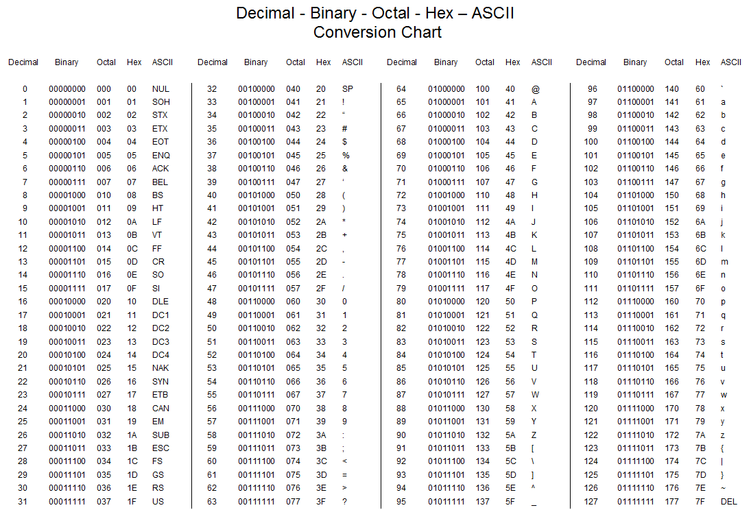
Converting binary numbers to decimal numbers¶

To convert from a binary number to a decimal number, we simple use the expression

d_{N-1}d_{N-2}\cdots d_2d_1d_0 = \sum_{n=0}^{N-1} d_n b^n\ .

(18)

As an example, we get that 1101₂ converts to

\begin{align} 1101_2 &= 1\cdot 2^3 + 1\cdot 2^2 + 0\cdot 2^1 + 1\cdot 2^0\\ &= 1 \cdot 8 + 1 \cdot 4 + 0\cdot 2 + 1\cdot 1\\ &= 13_{10}\ . \end{align}

(19)

Converting from decimal numbers to binary numbers is also possible, but is not covered here.

Adding binary numbers¶

You do it exactly as you learned in 2nd grade with decimal numbers. That is,

$0_2+0_2 = 0_2$
$0_2+1_2 = 1_2$
$1_2+1_2 = 0_2$ with 1₂ in carry

Using these three rules, we obtain $$ \begin{array}[t]{r} 0100\ 1001_2 \

\ 0111\ 1100_2 \ \hline 1100\ 0101_2 \end{array} $$

Example: Representing text using binary numbers¶

Example: Storing data on a disc¶

Information is stored by making tiny indentations known as pits on a disc.

A pit represents a 0
The opposite of a pit (called land) represents a 1

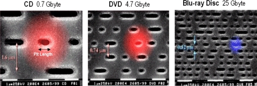
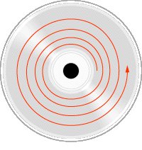
The binary data is stored along one long spiral on the disc.
CD: The spiral is 5.7 km long
DVD: The spiral is 12.3 km long
Blu-ray: The spiral is 28.4 km long
A laser is used for reading the binary data by following this spiral path.

Summary¶

A binary number
- only contains 0s and 1s
- consists of bits
A collection of eight bit is called a byte
Everything (numbers, text, images, video, audio, etc.) is stored and manipulated as binary numbers on a computer
The following slightly geeky joke is now funny ;)

There are 10 types of people in this world. Those who understand binary numbers and those who don’t!

Assignment¶

Bonus info:

With base $b=2$ , a binary number can be written as
$d_{N-1}d_{N-2}\cdots d_2d_1d_0 = \sum_{n=0}^{N-1} d_n b^n\ .$
(20)
G means billion (10⁹), M means million (10⁶), k means thousand (10³), and B means byte (8 bit)

Quantisation¶

In the next 20 minutes, you will learn

What quantisation is and why it is necessary
How you will typically do it
What signal-to-noise ratio (SNR) and dynamic range is

Example: Storing $\pi$ on a computer¶

How would you store $\pi$ (or other irrational numbers) on a computer?

It requires an infinite amount of memory to store $\pi$ on a computer.
Therefore, we have to store an approximation to $\pi$ with only a finite number of digits. Let us call this approximation $p$ .
The approximation error $e$ can be written as
$e = \pi-p\ .$
(21)

Example: Let $p$ contain only the first two digits of $\pi$ after the comma (i.e., $p=3.14$ ). Then

e = \pi-p = \pi-3.14 = 0.001592653589\ldots

(22)

We say that we have rounded of (or quantized) $\pi$ to its nearest two-digits-after-the-comma representation.

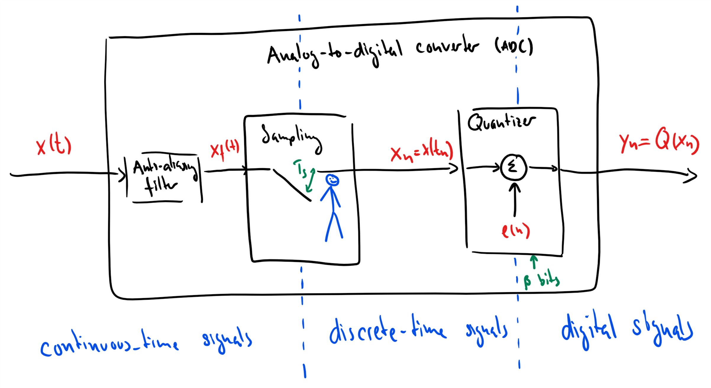
The need for quantisation¶

Sampling converts a continuous-time signal into a discrete-time signal. That is, we go from an infinite number of time values to a finite number of time values.

However, we also have to do something about the signal value $x(t_n)=x_n$ for every sampling time, so that we can store this number on the computer using a finite number of digits. This is called quantisation.

Uniform quantisation¶

Assume that we sample the signal value $x_n$ and that

the signal value is in the interval $(-\alpha,\alpha)$
we have $\beta$ bits available for storing this signal value. Note that we can represent $2^\beta$ different values with $\beta$ bits.

We now do the following.

Divide the interval $(-\alpha,\alpha)$ into $2^\beta$ equally large cells, each of size
$\Delta = \frac{\alpha-(-\alpha)}{2^\beta} = \frac{2\alpha}{2^\beta} = \frac{\alpha}{2^{\beta-1}}\ .$
(23)
Round (or quantise) the signal value $x_n$ to the value $y_n$ at the nearest cell boundary, i.e.,
$y_n = Q(x_n) = \Delta \left\lfloor\frac{x_n}{\Delta}\right\rceil = \Delta \left\lfloor\frac{x_n}{\Delta}+\frac{1}{2}\right\rfloor$
(24)
where $\lfloor\cdot\rceil$ and $\lfloor\cdot\rfloor$ refer to the rounding and flooring operations, respectively.

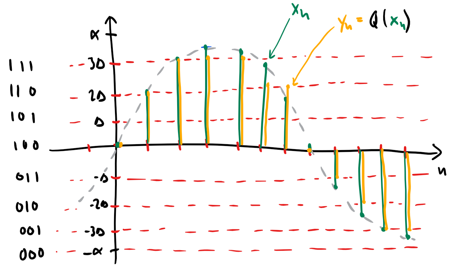
Example: 3 bit quantisation¶

In the figure below, the continuous-time signal (dashed gray) is first sampled (green) and then quantised (orange) using a three bit quantiser. The horisontal dashed red lines mark the quantisation levels. The final bit stream is

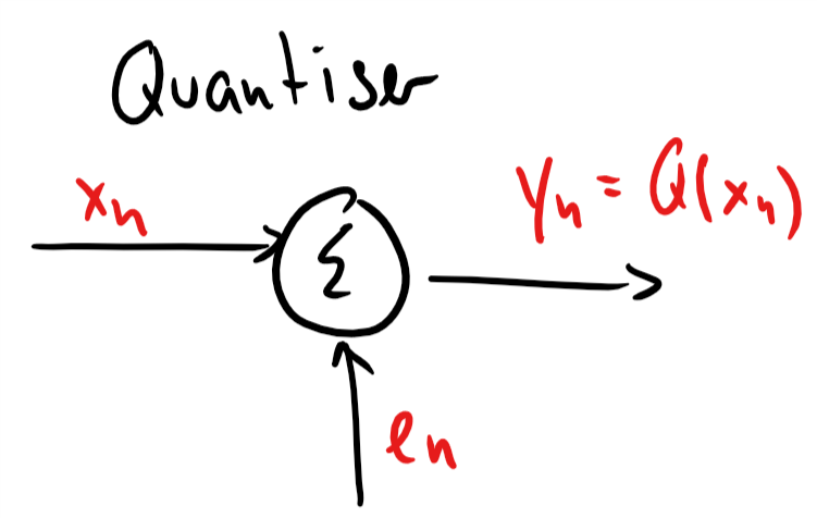
100\ 110\ 111\ 111\ 111\ 110\ 110\ 100\ 011\ 010\ 001\ 001\ .

(25)

Quantisation error¶

The quantisation error $e_n$ is the difference between the signal value $x_n$ and its rounded value $y_n=Q(x_n)$ , i.e.,

e_n = x_n-Q(x_n)\ .

(26)

We can rearrange this into

Q(x_n) = x_n+e_n\ .

(27)

That is, we can think of quantisation as adding an error to the signal value $x_n$ .

A measure of quantisation quality is how big the average power of $e_n$ is compared to the average power of $x_n$ . The average power of, e.g., $e_n$ is defined as

P_e = \frac{1}{N}\sum_{n=0}^{N-1} e_n^2\ .

(28)

If we define $P_x$ in a similar way, the signal-to-noise ratio (SNR) is defined as

\text{SNR} = 10\log_{10}\frac{P_x}{P_e}\ ,

(29)

and it is measured in decibel (dB).

Now, assume that

the signal values $x_n$ take on values in $(-\alpha,\alpha)$ equally often (a uniform distribution)
the quantisation errors $e_n$ take on values in $(-\Delta/2,\Delta/2)$ equally often (a uniform distribution)

We then get

\begin{align} P_x &= \frac{(2\alpha)^2}{12} = \frac{\alpha^2}{3}\\ P_e &= \frac{\Delta^2}{12} = \frac{1}{12}\left(\frac{\alpha}{2^{\beta-1}}\right)^2\ . \end{align}

(30)

These results can be derived by computing the variance of a uniform distribution.

Finally, we get the SNR

\begin{align} \text{SNR} &= 10\log_{10}\frac{P_x}{P_e} = 10\log_{10}\left(\frac{\alpha^2}{3}12\left(\frac{2^{\beta-1}}{\alpha}\right)^2\right)\\ &= 10\log_{10}\left(2^{2\beta}\right) = \beta 20 \log_{10} 2 \approx 6\beta\ . \end{align}

(31)

Thus, for every additional bit, the SNR is improved by approximately 6 dB.

Dynamic range¶

The dynamic range is the ratio between the loudest and softest values we can represent using a $\beta$ bit quantiser.

Softest value: 1
Loudest value: $2^\beta$

The dynamic range of a quantiser is thus

\text{DR} = 10\log_{10}\left(\left(\frac{2^\beta}{1}\right)^2\right) = 10\log_{10}\left(2^{2\beta}\right) = \beta 20 \log_{10} 2 \approx 6\beta\ .

(32)

Thus, we get a dynamic range of 96 dB for a 16 bit quantiser (typical CD quality) and 144 dB for a 24 bit quantiser. Note that the dynamic range of the human ear is approximately 120 dB.

Summary¶

A quantiser rounds the signal values to a value on a grid.
All the points of the grid can be represented using $\beta$ bits which results in $2^\beta$ possible values.
Quantisation introduces noise into the digital signal. The signal-to-noise ratio (SNR) describes how powerful the signal is compared to this quantisation noise.
The SNR (and dynamic range) depends on the number of bits used as
$\beta20\log_{10} \approx 6\beta\ .$
(33)

Assignment¶

Think of ways for increasing the dynamic range without increasing the number of the bits. Hint = Could non-uniform quantisation work?

Sampling and reconstruction

Sampling and reconstruction¶

Continuous-time signal¶

Sampling¶

Discrete-time signal¶

Reconstruction¶

Summary¶

Aliasing¶

Discrete-time sinusoid¶

What is Aliasing?¶

Nyquist-Shannon sampling theorem¶

Typical sampling frequencies used for recording audio¶

Anti-aliasing filter¶

Aliasing also occours in videos and images¶

Summary¶

Binary numbers¶

The decimal number systems¶

TODO The binary number system¶

Converting binary numbers to decimal numbers¶

Adding binary numbers¶

Example: Representing text using binary numbers¶

Example: Storing data on a disc¶

Summary¶

Assignment¶

Quantisation¶

Example: Storing π\piπ on a computer¶

The need for quantisation¶

Uniform quantisation¶

Example: 3 bit quantisation¶

Quantisation error¶

Dynamic range¶

Summary¶

Assignment¶

Example: Storing $\pi$ on a computer¶