![]()
Edge Impulse - Spectral Analysis Block#
Spectral Analysis Block#
EI Implementation_version >= 2 (Including Wavelets)
by Marcelo Rovai @ March23
FFT#
Statistical features (Time Domain) per axis/channel:#
After filtering via a Butterworth IIR filter (if enabled), the mean is subtracted from the signal. and are calculated:
RMS
Skewness
Kurtosis
Spectral features (Frequency Domain) per axis/channel:#
Spectral Power
Skewness
Kurtosis
Spectral Power#
The filtered signal is passed to the Spectral power section, which computes the FFT in order to compute the spectral features.
The window will be broken into frames (or “sub-windows”), and the FFT is calculated from each frame.
FFT length determines the number of FFT bins as well as the resolution of frequency peaks that you can separate.
The total number of Spectral Power features will change, depending on how you set the filter and FFT parameters. With No filtering, the number of features is 1/2 of FFT Length
https://docs.edgeimpulse.com/docs/edge-impulse-studio/processing-blocks/spectral-features
Wavelets#
In case of Wavelets, the extracted features are statistical features, crossing features and entropy features (14 per layer):
[11] Features: n5, n25, n75, n95, mean, median, standard deviation (std), variance (var) and root mean square (rms), kurtosis and skewness (skew) are calculated.[2] Features: Zero crossing rate (zcross) and mean crossing rate (mcross) are the times that the signal passes through the baseline (y = 0) and the average level (y = u) per unit time respectively[1] Feature: Entropy features are characteristic measure of signal complexity
All above 14 values are calculated for each Layer (including L0, the original signal)
[Inputs]: The Wavelet Decomposition level (1, 2, …) and what type of Wavelet (bior1.3, db2, …) to use should be defined. If for example, level 1 is chosen, L0 and L1 are used for feature calculationThe total number of features will change, depending on how you set the filter and the number of layers. For example, with [None] filtering, and Level [1], the number of features per axis will 14 x 2 (L0 and L1) = 28. For 6 axis, we will have a total of 168 features.
Statistical features#
Libraries#
import numpy as np
import matplotlib.pyplot as plt
import seaborn as sns
import math
from scipy.stats import skew, kurtosis
from scipy import signal
from scipy.signal import welch
from scipy.stats import entropy
from sklearn import preprocessing
!pip install pywavelets
import pywt
Collecting pywavelets
  Downloading pywavelets-1.8.0-cp311-cp311-manylinux_2_17_x86_64.manylinux2014_x86_64.whl.metadata (9.0 kB)
Requirement already satisfied: numpy<3,>=1.23 in /usr/local/lib/python3.11/dist-packages (from pywavelets) (1.26.4)
Downloading pywavelets-1.8.0-cp311-cp311-manylinux_2_17_x86_64.manylinux2014_x86_64.whl (4.5 MB)
   ━━━━━━━━━━━━━━━━━━━━━━━━━━━━━━━━━━━━━━━━ 4.5/4.5 MB 23.2 MB/s eta 0:00:00
?25hInstalling collected packages: pywavelets
Successfully installed pywavelets-1.8.0
plt.rcParams['figure.figsize'] = (12, 6)
plt.rcParams['lines.linewidth'] = 3
Functions#
def plot_data(sensors, axis, title):
    [plt.plot(x, label=y) for x,y in zip(sensors, axis)]
    plt.legend(loc='lower right')
    plt.title(title)
    plt.xlabel('#Sample')
    plt.ylabel('Value')
    plt.box(False)
    plt.grid()
    plt.show()
Clone the public project: https://studio.edgeimpulse.com/public/198358/latest
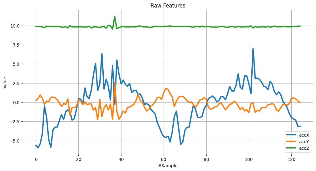
Get a datasample from accelerometers (2 seconds window; Sample frequency 62.5Hz)

f =  62.5  # Hertz
wind_sec = 2 # seconds
axis = ['accX', 'accY', 'accZ']
n_sensors = len(axis)
print (f'Frequency = {f}Hz')
print (f'Window = {wind_sec}s')
print (f'No Sensors = {len(axis)}')
Frequency = 62.5Hz
Window = 2s
No Sensors = 3
data=[-5.6330, 0.2376, 9.8701, -5.9442, 0.4830, 9.8701, -5.4217, 0.9433, 9.8521, -4.1474, 0.5261, 9.8246, -0.4896, -0.2592, 9.7217, -1.9465, 0.1472, 9.9108, -4.8261, 0.0449, 9.8964, -5.8861, 0.6291, 9.8988, -3.6248, 0.6734, 9.8731, -3.2585, 0.5866, 9.8491, -3.2304, 0.3358, 9.9000, -2.4187, -0.1071, 9.8593, -1.6017, -0.5381, 9.7941, -2.2577, -0.1760, 9.7803, -1.2438, -0.2873, 9.8438, -0.9978, 0.4076, 9.6696, -1.3210, -1.6514, 9.9754, -2.3337, -0.6740, 9.8084, -2.1272, -0.7195, 9.8330, -0.9792, -0.5584, 9.8013, 0.4615, 0.3041, 9.8306, 0.4076, 0.1861, 9.8390, -0.2682, -0.3226, 9.8043, 1.8477, 0.0377, 9.7977, 0.7560, -0.3166, 9.8072, 0.4764, -0.2215, 9.9084, 1.5724, -0.2274, 9.6744, 3.5195, -1.0169, 9.8234, 5.0560, -0.7021, 9.8270, 1.5137, -2.2853, 9.7875, 2.4044, 0.3328, 9.7582, 6.3111, -1.8765, 9.8288, 1.7196, -0.7302, 9.8623, 2.9999, -0.3268, 9.6516, 2.0800, -1.0092, 10.0347, 0.2867, -0.2406, 9.9653, 4.7908, -2.2739, 9.5343, -0.2652, 2.5833, 11.1749, 5.4857, -1.2103, 9.5672, 3.6763, -2.2194, 9.7282, 2.3888, -1.7867, 9.8276, 2.8802, -1.1588, 9.8970, 2.3320, -1.4042, 9.7977, 2.0650, -0.6913, 9.8228, 2.4505, -0.6297, 9.8025, 1.2851, -0.4441, 9.8354, 1.5113, -0.2927, 9.8282, 1.5616, 0.2173, 9.8090, 1.0199, 0.9936, 9.9192, 1.0570, 0.2257, 9.9317, 0.5112, 0.0192, 9.8336, -0.2867, -0.6770, 9.8180, -0.2017, -1.1558, 9.8192, -0.3322, -0.9535, 9.7665, -0.9379, -0.4998, 9.7588, -1.2540, -0.3106, 9.8240, -1.5287, 0.0634, 9.9108, -2.6606, 0.5758, 9.8779, -3.2723, 0.6482, 9.8761, -4.0121, 0.3585, 9.8462, -4.4945, 1.2276, 9.9042, -4.5849, 1.7909, 9.9000, -4.4335, 1.6777, 9.9060, -5.1697, 1.1486, 9.9377, -3.9115, 0.7159, 9.8857, -1.8699, -0.5561, 9.8845, -1.1618, 0.1490, 9.8497, -3.2902, 0.6542, 9.8683, -5.5055, 0.7530, 9.8845, -5.1739, 0.7482, 9.8821, -3.6524, 0.5028, 9.8641, -3.2645, 0.1778, 9.8629, -3.2423, -0.0048, 9.8970, -1.6729, 0.0311, 9.8013, -0.3244, -0.3364, 9.7839, -0.9966, -0.6692, 9.8761, -1.9950, -0.2113, 9.8964, -2.0075, 0.3011, 9.7965, -1.8633, 0.3370, 9.9288, -0.8739, 0.5926, 9.8162, -0.4046, 0.3974, 9.8665, 0.4830, -0.6788, 9.8659, 0.6201, -0.8948, 9.8312, 0.8027, -0.8200, 9.7725, 0.5213, -0.6087, 9.8126, 0.0275, -0.5608, 9.7713, 0.2412, -0.1885, 9.8665, 0.7596, -0.0581, 9.8521, 0.6907, -0.5483, 9.8881, 0.3244, -0.9978, 9.7773, 1.0576, -0.6584, 9.7887, 2.0722, -0.2753, 9.8120, 1.4647, -0.2221, 9.8928, 1.4617, 0.1341, 9.8120, 2.2188, -0.0329, 9.7773, 3.6859, -0.5171, 9.9084, 1.9172, -0.9744, 9.8019, 1.7095, -0.6734, 9.8061, 3.4327, -1.1205, 9.8372, 3.4399, -0.9679, 9.8342, 2.4307, -1.3473, 9.8240, 1.1283, -0.1945, 9.9479, 6.9707, -0.0946, 9.6744, 3.0957, -1.3120, 9.8617, 3.1448, -1.0924, 9.7701, 2.9862, -1.1349, 9.8144, 2.6073, -0.7344, 9.8025, 2.0824, -0.6955, 9.8396, 1.9932, -0.6812, 9.7809, 1.6640, -0.3089, 9.8845, 2.6833, -0.2879, 9.7929, 2.3272, -0.1706, 9.8288, 1.3761, -0.3537, 9.9228, 0.9643, -1.0145, 9.8318, 1.3420, -1.1498, 9.8360, 0.9942, -0.7326, 9.8288, 0.1395, -0.3202, 9.8695, -0.2993, -0.3220, 9.8527, -0.6967, -0.3980, 9.8360, -1.4706, -0.1879, 9.8342, -1.9974, 0.5267, 9.8474, -2.1883, 0.5584, 9.8695, -2.3409, 0.4447, 9.8815, -3.1214, 0.1730, 9.9168, -3.1502, -0.0156, 9.9174]
No_raw_features = len(data)
N = int(No_raw_features/n_sensors)
print (f"No. raw features: {No_raw_features}; N= {N} (number of features per axix)")
No. raw features: 375; N= 125 (number of features per axix)
# Processed Features
features = [2.7322, -0.0978, -0.3813, 2.3980, 3.8924, 24.6841, 9.6303, 8.4867, 7.7793, 2.9963, 5.6242, 3.4198, 4.2735, 0.7833, 0.1735, 1.1696, 0.9426, -0.8039, 5.4290, 0.9990, 1.0315, 0.9459, 1.8117, 0.9088, 1.3302, 3.1120, 0.1383, 6.8629, 65.3726, 0.3117, -1.3812, 0.0606, 0.0570, 0.0567, 0.0976, 0.1940, 0.2574, 0.2083, 0.1660]
N_feat = len(features)
N_feat_axis = int(N_feat/n_sensors)
print(f' - Total Number of features without filtering: {N_feat}')
print(f' - Total Number of Statistical features : {3*n_sensors}')
print(f' - Total Number of Spectral features : {N_feat-3*n_sensors}')
print(f' - Total Number of features per axis: {N_feat_axis}')
 - Total Number of features without filtering: 39
 - Total Number of Statistical features : 9
 - Total Number of Spectral features : 30
 - Total Number of features per axis: 13
3 Statistical features (time) per axis –> Total: 9 features
8 Spectral Power Features (Freq) per axis –> Total: 24 features
2 Spectral Skew/Kurtosis (freq) per axis -> Total: 6 features
Total Processed Features = 9+24+6 = 39
Features per axix: [rms] [skew] [kurtosis] [spectral skew] [spectral kurtosis] [Spectral Power 1] ... [Spectral Power 8]
Split raw data per sensor#
accX = data[0::3]
accY = data[1::3]
accZ = data[2::3]
sensors = [accX, accY, accZ]
plot_data(sensors, axis, 'Raw Features')
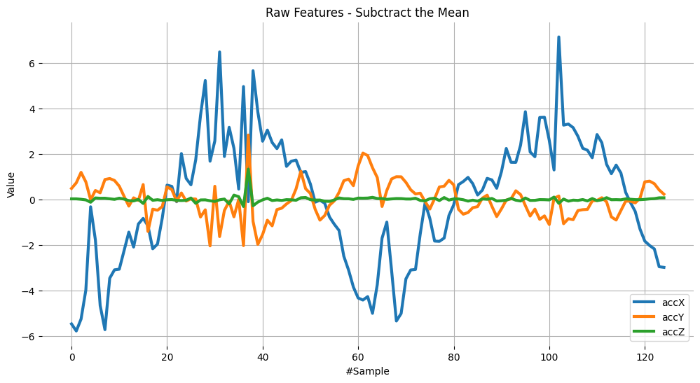
Subtrating the mean from data#
Subtracting the mean from a set of data is a common data pre-processing step in statistics and machine learning. The purpose of subtracting the mean from data is to center the data around zero. This is important because it can reveal patterns and relationships that might be hidden if the data is not centered.
Here are some specific reasons why subtracting the mean can be useful:
It simplifies analysis: By centering the data, the mean becomes zero, which can make some calculations simpler and easier to interpret.
It removes bias: If the data has a bias, subtracting the mean can remove that bias and allow for more accurate analysis.
It can reveal patterns: Centering the data can help reveal patterns that might be hidden if the data is not centered. For example, if you are analyzing a time series dataset, centering the data can help you identify trends over time.
It can improve performance: In some machine learning algorithms, centering the data can improve performance by reducing the influence of outliers and making the data more easily comparable. Overall, subtracting the mean is a simple but powerful technique that can be used to improve the analysis and interpretation of data.
dtmean = [(sum(x)/len(x)) for x in sensors]
[print('mean_'+x+'= ', round(y, 4)) for x,y in zip(axis, dtmean)][0]
mean_accX=  -0.1646
mean_accY=  -0.2438
mean_accZ=  9.8472
accX = [(x - dtmean[0]) for x in accX]
accY = [(x - dtmean[1]) for x in accY]
accZ = [(x - dtmean[2]) for x in accZ]
sensors = [accX, accY, accZ]
plot_data(sensors, axis, 'Raw Features - Subctract the Mean')
RMS Calculation#
The RMS value of a set of values (or a continuous-time waveform) is the square root of the arithmetic mean of the squares of the values, or the square of the function that defines the continuous waveform. In physics, the RMS current value can also be defined as the “value of the direct current that dissipates the same power in a resistor.”
In the case of a set of n values \(\{x_{1},x_{2},\dots ,x_{n}\}\), the RMS is:
\(\displaystyle x_{\text{RMS}}={\sqrt {{\frac {1}{n}}\left(x_{1}^{2}+x_{2}^{2}+\cdots +x_{n}^{2}\right)}}.\)
NOTE that the RMS value is different for original raw data and after subtracting the mean
# Using numpy and standartized data (subtracting mean)
rms = [np.sqrt(np.mean(np.square(x))) for x in sensors]
[print('rms_'+x+'= ', round(y, 4)) for x,y in zip(axis, rms)][0]
rms_accX=  2.7322
rms_accY=  0.7833
rms_accZ=  0.1383
# Compare with Edge Impulse result features
features[0:N_feat:N_feat_axis]
[2.7322, 0.7833, 0.1383]
Skewness and kurtosis calculation#
In statistics, skewness and kurtosis are two ways to measure the shape of a distribution.
Skewness is a measure of the asymmetry of a distribution. This value can be positive or negative.

A negative skew indicates that the tail is on the left side of the distribution, which extends towards more negative values.
A positive skew indicates that the tail is on the right side of the distribution, which extends towards more positive values.
A value of zero indicates that there is no skewness in the distribution at all, meaning the distribution is perfectly symmetrical.
Kurtosis is a measure of whether or not a distribution is heavy-tailed or light-tailed relative to a normal distribution.

The kurtosis of a normal distribution is 0.
If a given distribution has a kurtosis is negative, it is said to be playkurtic, which means it tends to produce fewer and less extreme outliers than the normal distribution.
If a given distribution has a kurtosis positive, it is said to be leptokurtic, which means it tends to produce more outliers than the normal distribution.
NOTE that the Skewness and Kurtosis values are the same for original raw data and after subtracting the mean
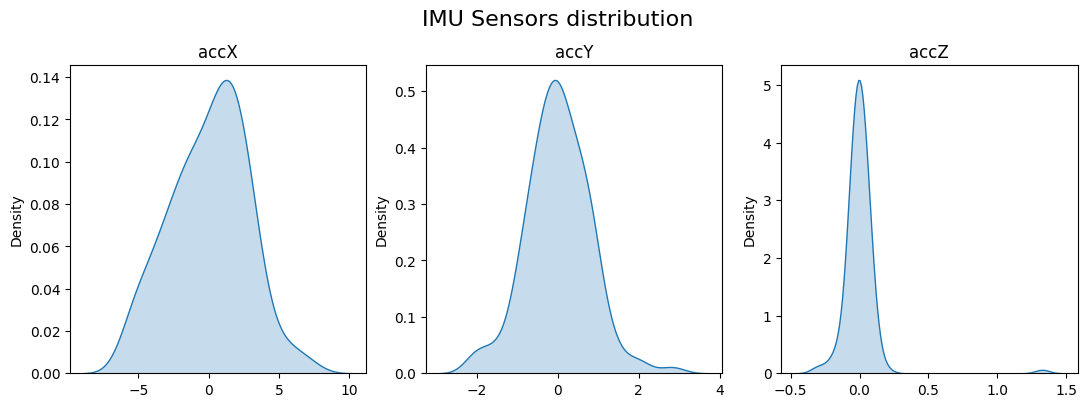
Let’s see the data distribution and the Skewness and kurtosis calculation
fig, axes = plt.subplots(nrows=1, ncols=3, figsize=(13, 4))
sns.kdeplot(accX, fill=True, ax=axes[0])
sns.kdeplot(accY, fill=True, ax=axes[1])
sns.kdeplot(accZ, fill=True, ax=axes[2])
axes[0].set_title('accX')
axes[1].set_title('accY')
axes[2].set_title('accZ')
plt.suptitle('IMU Sensors distribution', fontsize=16, y=1.02)
plt.show()
skew = [skew(x, bias=False) for x in sensors]
[print('skew_'+x+'= ', round(y, 4)) for x,y in zip(axis, skew)][0]
skew_accX=  -0.099
skew_accY=  0.1756
skew_accZ=  6.9463
# Compare with Edge Impulse result features
features[1:N_feat:N_feat_axis]
[-0.0978, 0.1735, 6.8629]
kurt = [kurtosis(x, bias=False) for x in sensors]
[print('kurt_'+x+'= ', round(y, 4)) for x,y in zip(axis, kurt)][0]
kurt_accX=  -0.3475
kurt_accY=  1.2673
kurt_accZ=  68.1123
# Compare with Edge Impulse result features
features[2:N_feat:N_feat_axis]
[-0.3813, 1.1696, 65.3726]
Spectral features#
FFT_Lenght = 16
fs = f
print (f"Sample Frequency: {f}Hz")
Sample Frequency: 62.5Hz
Once the sampled window usually is larger than the FFT size, the window will be broken into frames (or “sub-windows”), and the FFT is calculated from each frame.
FFT length - The FFT size. This determines the number of FFT bins as well as the resolution of frequency peaks that you can separate. A lower number means more signals will average together in the same FFT bin, but also reduces the number of features and model size. A higher number will separate more signals into separate bins, but generates a larger model.
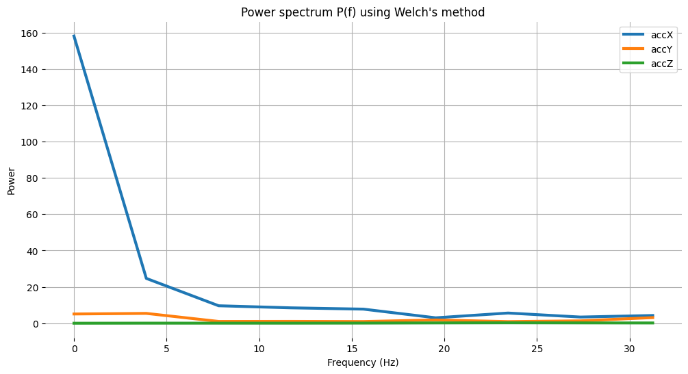
Spectral Power - Welch’s method#
https://docs.scipy.org/doc/scipy-0.14.0/reference/generated/scipy.signal.welch.html
To split the signal on frequency domain in bins and calculate the power spectrum for each bin, we should use a method called Welch’s method.
This method divides the signal into overlapping segments, applies a window function to each segment, computes the periodogram of each segment using DFT, and averages them to obtain a smoother estimate of the power spectrum.
# Function used by Edge Impulse insteady scipy.signal.welch().
def welch_max_hold(fx, sampling_freq, nfft, n_overlap):
    n_overlap = int(n_overlap)
    spec_powers = [0 for _ in range(nfft//2+1)]
    ix = 0
    while ix <= len(fx):
        # Slicing truncates if end_idx > len, and rfft will auto zero pad
        fft_out = np.abs(np.fft.rfft(fx[ix:ix+nfft], nfft))
        spec_powers = np.maximum(spec_powers, fft_out**2/nfft)
        ix = ix + (nfft-n_overlap)
    return np.fft.rfftfreq(nfft, 1/sampling_freq), spec_powers
fax,Pax = welch_max_hold(accX, fs, FFT_Lenght, 0)
fay,Pay = welch_max_hold(accY, fs, FFT_Lenght, 0)
faz,Paz = welch_max_hold(accZ, fs, FFT_Lenght, 0)
specs = [Pax, Pay, Paz ]
Note that since we subtract the mean at the begining, bin 0 (DC) will always be ~0, so we skip it (p[1:])
# Plot power spectrum versus frequency
# Since we subtract the mean at the begining, bin 0 (DC) will always be ~0, so skip it
plt.plot(fax,Pax, label='accX')
plt.plot(fay,Pay, label='accY')
plt.plot(faz,Paz, label='accZ')

plt.legend(loc='upper right')
plt.xlabel('Frequency (Hz)')
#plt.ylabel('PSD [V**2/Hz]')
plt.ylabel('Power')
plt.title('Power spectrum P(f) using Welch\'s method')
plt.grid()
plt.box(False)
plt.show()
print("\nCalculated Spectral Power features for accX:")
[print(round(x, 4)) for x in Pax[1:]][0]
Calculated Spectral Power features for accX:
24.6844
9.6304
8.4865
7.7794
2.9964
5.6242
3.4198
4.2736
print("\nCalculated Spectral Power features for accY:")
[print(round(x, 4)) for x in Pay[1:]][0]
Calculated Spectral Power features for accY:
5.4289
0.999
1.0315
0.9458
1.8116
0.9088
1.3301
3.1121
print("\nCalculated Spextral Power features for accZ:")
[print(round(x, 4)) for x in Paz[1:]][0]
Calculated Spextral Power features for accZ:
0.0606
0.057
0.0567
0.0976
0.194
0.2574
0.2083
0.166
Spectral Skewness and Kurtosis#
If you got an error, import the libraries again
from scipy.stats import skew # Import the skew function explicitly
spec_skew = [skew(x, bias=False) for x in specs]
[print('spectral_skew_'+x+'= ', round(y, 4)) for x,y in zip(axis, spec_skew)][0]
spectral_skew_accX=  2.9069
spectral_skew_accY=  1.1426
spectral_skew_accZ=  0.3781
spec_kurtosis = [kurtosis(x, bias=False) for x in specs]
[print('spectral_kurtosis_'+x+'= ', round(y, 4)) for x,y in zip(axis, spec_kurtosis)][0]
spectral_kurtosis_accX=  8.5569
spectral_kurtosis_accY=  -0.3886
spectral_kurtosis_accZ=  -1.4874
List Spectral features per axis and compare with EI#
print("EI Processed Spectral features (accX): ")
print(features[3:N_feat_axis][0:])
print("\nCalculated features:")
print (round(spec_skew[0],4))
print (round(spec_kurtosis[0],4))
[print(round(x, 4)) for x in Pax[1:]][0]
EI Processed Spectral features (accX):
[2.398, 3.8924, 24.6841, 9.6303, 8.4867, 7.7793, 2.9963, 5.6242, 3.4198, 4.2735]

Calculated features:
2.9069
8.5569
24.6844
9.6304
8.4865
7.7794
2.9964
5.6242
3.4198
4.2736
print("EI Processed Spectral features (accY): ")
print(features[16:26][0:]) #13: 3+N_feat_axis;  26 = 2x N_feat_axis
print("\nCalculated features:")
print (round(spec_skew[1],4))
print (round(spec_kurtosis[1],4))
[print(round(x, 4)) for x in Pay[1:]][0]
EI Processed Spectral features (accY):
[0.9426, -0.8039, 5.429, 0.999, 1.0315, 0.9459, 1.8117, 0.9088, 1.3302, 3.112]

Calculated features:
1.1426
-0.3886
5.4289
0.999
1.0315
0.9458
1.8116
0.9088
1.3301
3.1121
print("EI Processed Spectral features (accZ): ")
print(features[29:][0:]) #29: 3+(2*N_feat_axis);
print("\nCalculated features:")
print (round(spec_skew[2],4))
print (round(spec_kurtosis[2],4))
[print(round(x, 4)) for x in Paz[1:]][0]
EI Processed Spectral features (accZ):
[0.3117, -1.3812, 0.0606, 0.057, 0.0567, 0.0976, 0.194, 0.2574, 0.2083, 0.166]

Calculated features:
0.3781
-1.4874
0.0606
0.057
0.0567
0.0976
0.194
0.2574
0.2083
0.166
Wavelets#
Wavelet is a powerful technique that is especially useful for analyzing signals with transient features or abrupt changes, such as spikes or edges, which are difficult to analyze with traditional Fourier-based techniques.
Wavelet transforms work by breaking down a signal into different frequency components and analyzing them individually. The transformation is achieved by convolving the signal with a wavelet function, which is a small waveform that is centered at a specific time and frequency. This process effectively decomposes the signal into different frequency bands, each of which can be analyzed separately.
One of the key benefits of wavelet transforms is that they allow for time-frequency analysis, which means that they can reveal the frequency content of a signal as it changes over time. This makes them particularly useful for analyzing non-stationary signals, which vary over time.
Wavelets have many practical applications, including signal and image compression, denoising, feature extraction, and image processing.
Let’s select Wavelet on Spectral Features block

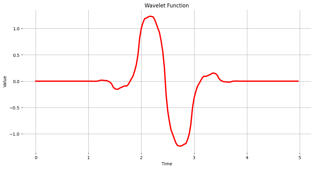
The Wavelet Fuction#
wavelet_name='bior1.3'
num_layer = 1
wavelet = pywt.Wavelet(wavelet_name)
[phi_d,psi_d,phi_r,psi_r,x] = wavelet.wavefun(level=5)
plt.plot(x, psi_d, color='red')
plt.title('Wavelet Function')
plt.ylabel('Value')
plt.xlabel('Time')
plt.grid()
plt.box(False)
plt.show()
Processed Features#
features = [3.6251, 0.0615, 0.0615, -7.3517, -2.7641, 2.8462, 5.0924, 0.4063, -0.2133, 3.8473, 15.0327, 3.8532, -0.2905, -0.7966, 3.3929, 0.5231, 0.5538, -1.3234, -0.2743, 0.5206, 1.4599, 0.1350, 0.1264, 0.9544, 0.9250, 0.9627, 0.6358, 3.0473, 3.6597, 0.3077, 0.3077, -1.3234, -0.6492, 0.7844, 1.3610, 0.0659, 0.0276, 0.9345, 0.8868, 0.9349, 0.2807, -0.0589, 3.1609, 0.5385, 0.5385, -0.5356, -0.2709, 0.2298, 0.8409, -0.0830, -0.0377, 0.6040, 0.3706, 0.6052, -2.2028, 13.7548, 3.1061, 0.4000, 0.3692, -0.1126, -0.0494, 0.0347, 0.1022, -0.0137, 0.0025, 0.1053, 0.0113, 0.1053, 4.3072, 26.4113, 2.6219, 0.4462, 0.3385, -0.1122, -0.0250, 0.0233, 0.0793, 0.0008, -0.0183, 0.1529, 0.0237, 0.1540, -6.3676, 44.9559]
N_feat = len(features)
N_feat_axis = int(N_feat/n_sensors)
print(f' - Total Number of features without filtering: {N_feat}')
print(f' - Total Number of features per layer: {int(N_feat/(num_layer+1))}')
print(f' - Total Number of features per axis per layer: {N_feat_axis}')
 - Total Number of features without filtering: 84
 - Total Number of features per layer: 42
 - Total Number of features per axis per layer: 28
It is possible to calculate the maximum number of Wavelet decomposition levels.
pywt.dwt_max_level(len(accX), wavelet_name)
4
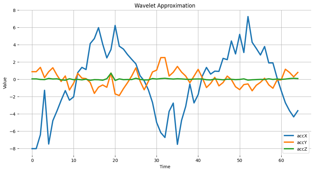
Wavelet Analysis#
Wavelet analysis decomposes a signal (accX, accY and accZ) into different frequency components using a set of filters applied to the signal, which separates these components into low-frequency (slowly varying parts of the signal containing long-term patterns), here accX_l1, accY_l1, accZ_l1 and, high-frequency (rapidly varying parts of the signal containing short-term patterns) components, here accX_d1, accY_d1, accZ_d1, allowing for the extraction of features for further analysis or classification. Only the low frequency components will be used. In this example we are assuming only one level (Single level Discrete Wavelet Transform), where the function will return a tupple. With a multilevel decomposition, the “Multilevel 1D Discrete Wavelet Transform”, the result will be a list. Discrete Wavelet Transform (DWT)
(accX_l1, accX_d1) = pywt.dwt(accX, wavelet_name)
(accY_l1, accY_d1) = pywt.dwt(accY, wavelet_name)
(accZ_l1, accZ_d1) = pywt.dwt(accZ, wavelet_name)
sensors_l1 = [accX_l1, accY_l1, accZ_l1]
# Plot power spectrum versus frequency
# Since we subtract the mean at the begining, bin 0 (DC) will always be ~0, so skip it
plt.plot(accX_l1, label='accX')
plt.plot(accY_l1, label='accY')
plt.plot(accZ_l1, label='accZ')
plt.legend(loc='lower right')
plt.xlabel('Time')
plt.ylabel('Value')
plt.title('Wavelet Approximation')
plt.grid()
plt.box(False)
plt.show()
Feature Extraction#
Basic Statistical Features#
def calculate_statistics(signal):
    n5 = np.percentile(signal, 5)
    n25 = np.percentile(signal, 25)
    n75 = np.percentile(signal, 75)
    n95 = np.percentile(signal, 95)
    median = np.percentile(signal, 50)
    mean = np.mean(signal)
    std = np.std(signal)
    var = np.var(signal)
    rms = np.sqrt(np.mean(np.square(signal)))
    return [n5, n25, n75, n95, median, mean, std, var, rms]
stat_feat_l0 = [calculate_statistics(x) for x in sensors]
stat_feat_l1 = [calculate_statistics(x) for x in sensors_l1]
print (f"feat_l0 or l_1 has {len(stat_feat_l0[0])} statistical features for each of the {len(stat_feat_l0)} axis")
feat_l0 or l_1 has 9 statistical features for each of the 3 axis
skew_l0 = [skew(x, bias=False) for x in sensors]
skew_l1 = [skew(x, bias=False) for x in sensors_l1]
kurtosis_l0 = [kurtosis(x, bias=False) for x in sensors]
kurtosis_l1 = [kurtosis(x, bias=False) for x in sensors_l1]
Crossings#
Zero crossing (zcross) is the number of times the wavelet coefficient crosses the zero axis. It can be used as a measure of the frequency content of the signal since high-frequency signals tend to have more zero crossings than low-frequency signals.
Mean crossing (mcross), on the other hand, is the number of times the wavelet coefficient crosses the mean of the signal. It can be used as a measure of the amplitude of the signal since high-amplitude signals tend to have more mean crossings than low-amplitude signals.
def getZeroCrossingRate(arr):
    my_array = np.array(arr)
    zcross = float("{0:.2f}".format((((my_array[:-1] * my_array[1:]) < 0).sum())/len(arr)))
    return zcross

def getMeanCrossingRate(arr):
    mcross = getZeroCrossingRate(np.array(arr) - np.mean(arr))
    return mcross
def calculate_crossings(list):
    zcross=[]
    mcross=[]
    for i in range(len(list)):
        zcross_i = getZeroCrossingRate(list[i])
        zcross.append(zcross_i)
        mcross_i = getMeanCrossingRate(list[i])
        mcross.append(mcross_i)
    return zcross, mcross
calculate_crossings(sensors_l1)
([0.06, 0.31, 0.4], [0.06, 0.31, 0.37])
cross_l0 = calculate_crossings(sensors)
cross_l1 = calculate_crossings(sensors_l1)
Entropy#
In wavelet analysis, entropy refers to the degree of disorder or randomness in the distribution of wavelet coefficients. Here we used Shannon entropy, that is a measure of the amount of uncertainty or randomness in a signal. It is calculated as the negative sum of the probabilities of the different possible outcomes of the signal multiplied by their logarithm base 2. In the context of wavelet analysis, Shannon entropy can be used to measure the complexity of the signal, with higher values indicating greater complexity.
def calculate_entropy(signal, base=None):
    value, counts = np.unique(signal, return_counts=True)
    return entropy(counts, base=base)
entropy_l0 = [calculate_entropy(x) for x in sensors]
entropy_l1 = [calculate_entropy(x) for x in sensors_l1]
List all weavelets features and create a list by layers#
L1_features_names = ["L1-n5", "L1-n25", "L1-n75", "L1-n95", "L1-median", "L1-mean", "L1-std", "L1-var", "L1-rms", "L1-skew", "L1-Kurtosis", "L1-zcross", "L1-mcross", "L1-entropy"]
L0_features_names = ["L0-n5", "L0-n25", "L0-n75", "L0-n95", "L0-median", "L0-mean", "L0-std", "L0-var", "L0-rms", "L0-skew", "L0-Kurtosis", "L0-zcross", "L0-mcross", "L0-entropy"]
len(L1_features_names)
14
all_feat_l0 = []
for i in range(len(axis)):
    feat_l0 = stat_feat_l0[i]+[skew_l0[i]]+[kurtosis_l0[i]]+[cross_l0[0][i]]+[cross_l0[1][i]]+[entropy_l0[i]]
    [print(axis[i]+' '+x+'= ', round(y, 4)) for x,y in zip(L0_features_names, feat_l0)][0]
    all_feat_l0.append(feat_l0)
all_feat_l0 = [item for sublist in all_feat_l0 for item in sublist]
print(f"\nAll L0 Features = {len(all_feat_l0)}")
accX L0-n5=  -4.9364
accX L0-n25=  -1.8429
accX L0-n75=  1.8842
accX L0-n95=  3.8096
accX L0-median=  0.4058
accX L0-mean=  -0.0
accX L0-std=  2.7322
accX L0-var=  7.4651
accX L0-rms=  2.7322
accX L0-skew=  -0.099
accX L0-Kurtosis=  -0.3475
accX L0-zcross=  0.06
accX L0-mcross=  0.06
accX L0-entropy=  4.8283
accY L0-n5=  -1.149
accY L0-n25=  -0.4475
accY L0-n75=  0.4814
accY L0-n95=  1.1491
accY L0-median=  -0.0315
accY L0-mean=  0.0
accY L0-std=  0.7833
accY L0-var=  0.6136
accY L0-rms=  0.7833
accY L0-skew=  0.1756
accY L0-Kurtosis=  1.2673
accY L0-zcross=  0.29
accY L0-mcross=  0.29
accY L0-entropy=  4.8283
accZ L0-n5=  -0.1242
accZ L0-n25=  -0.0429
accZ L0-n75=  0.0349
accZ L0-n95=  0.0839
accZ L0-median=  -0.0112
accZ L0-mean=  0.0
accZ L0-std=  0.1383
accZ L0-var=  0.0191
accZ L0-rms=  0.1383
accZ L0-skew=  6.9463
accZ L0-Kurtosis=  68.1123
accZ L0-zcross=  0.35
accZ L0-mcross=  0.35
accZ L0-entropy=  4.5649

All L0 Features = 42
all_feat_l1 = []
for i in range(len(axis)):
    feat_l1 = stat_feat_l1[i]+[skew_l1[i]]+[kurtosis_l1[i]]+[cross_l1[0][i]]+[cross_l1[1][i]]+[entropy_l1[i]]
    [print(axis[i]+' '+x+'= ', round(y, 4)) for x,y in zip(L1_features_names, feat_l1)][0]
    all_feat_l1.append(feat_l1)
all_feat_l1 = [item for sublist in all_feat_l1 for item in sublist]
print(f"\nAll L1 Features = {len(all_feat_l1)}")
accX L1-n5=  -7.3516
accX L1-n25=  -2.7641
accX L1-n75=  2.8462
accX L1-n95=  5.0924
accX L1-median=  0.4064
accX L1-mean=  -0.2133
accX L1-std=  3.8473
accX L1-var=  14.8015
accX L1-rms=  3.8532
accX L1-skew=  -0.2975
accX L1-Kurtosis=  -0.7631
accX L1-zcross=  0.06
accX L1-mcross=  0.06
accX L1-entropy=  4.1744
accY L1-n5=  -1.3234
accY L1-n25=  -0.6492
accY L1-n75=  0.7844
accY L1-n95=  1.361
accY L1-median=  0.0659
accY L1-mean=  0.0276
accY L1-std=  0.9345
accY L1-var=  0.8732
accY L1-rms=  0.9349
accY L1-skew=  0.2874
accY L1-Kurtosis=  0.0347
accY L1-zcross=  0.31
accY L1-mcross=  0.31
accY L1-entropy=  4.1317
accZ L1-n5=  -0.1126
accZ L1-n25=  -0.0493
accZ L1-n75=  0.0348
accZ L1-n95=  0.1022
accZ L1-median=  -0.0137
accZ L1-mean=  0.0025
accZ L1-std=  0.1053
accZ L1-var=  0.0111
accZ L1-rms=  0.1053
accZ L1-skew=  4.4095
accZ L1-Kurtosis=  28.6586
accZ L1-zcross=  0.4
accZ L1-mcross=  0.37
accZ L1-entropy=  4.1531

All L1 Features = 42
feat = all_feat_l0+all_feat_l1
len(feat)
84