Lecture 3: The Fourier Transform#
Signal Processing for Interactive Systems
Cumhur Erkut (cer@create.aau.dk)
Aalborg University Copenhagen.
Last edited: 2025-02-25
The discrete-time Fourier transform#
In this part, you will learn
why it is important to look at signals in the frequency domain
what the DTFT is
how you can visualise noise removal in the frequency domain
🔈 Understanding the DFT and the FFT (20 minutes)
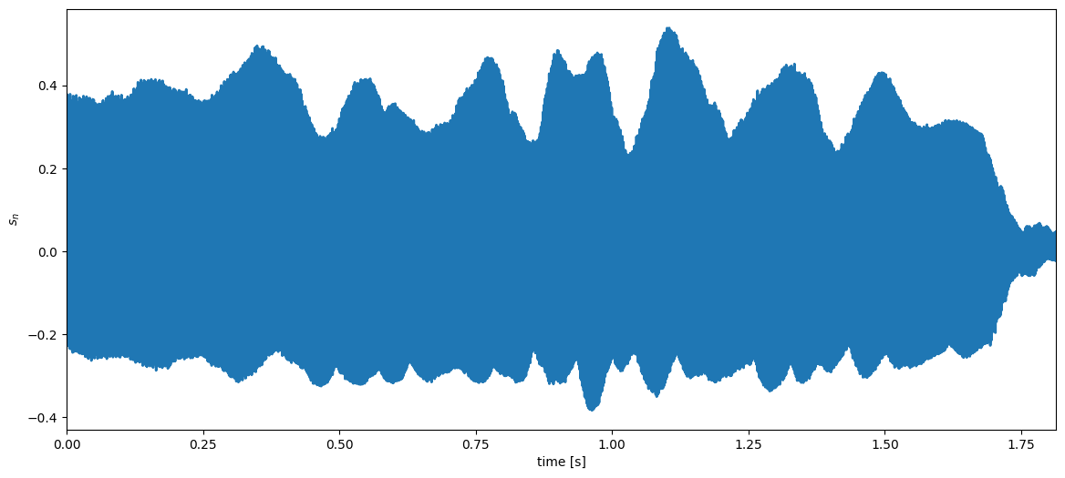
Example: analysing a trumpet signal Suppose that we record a trumpet signal \(s_n\) for \(n=0,1,2,\ldots,N-1\).

try:
  import google.colab
  IN_COLAB = True
  !mkdir -p data
  !wget https://raw.githubusercontent.com/SMC-AAU-CPH/med4-ap-jupyter/main/lecture7_Fourer_Transfom/data/trumpet.wav -P data
  !wget https://raw.githubusercontent.com/SMC-AAU-CPH/med4-ap-jupyter/main/lecture7_Fourer_Transfom/data/trumpetFull.wav -P data
except:
  IN_COLAB = False


# %matplotlib inline
import numpy as np
import matplotlib.pyplot as plt
import scipy.io.wavfile as wave
import IPython.display as ipd
import librosa

# If needed you can load the trumpet full audio file, and crop the beginning for a single note as trumpet.wav
# audio_data, sampling_rate = librosa.load(librosa.ex('trumpet'))
--2025-02-25 10:06:35--  https://raw.githubusercontent.com/SMC-AAU-CPH/med4-ap-jupyter/main/lecture7_Fourer_Transfom/data/trumpet.wav
Resolving raw.githubusercontent.com (raw.githubusercontent.com)... 185.199.108.133, 185.199.109.133, 185.199.110.133, ...
Connecting to raw.githubusercontent.com (raw.githubusercontent.com)|185.199.108.133|:443... connected.
HTTP request sent, awaiting response... 200 OK
Length: 160044 (156K) [audio/wav]
Saving to: ‘data/trumpet.wav’

trumpet.wav         100%[===================>] 156.29K  --.-KB/s    in 0.03s

2025-02-25 10:06:35 (4.66 MB/s) - ‘data/trumpet.wav’ saved [160044/160044]

--2025-02-25 10:06:35--  https://raw.githubusercontent.com/SMC-AAU-CPH/med4-ap-jupyter/main/lecture7_Fourer_Transfom/data/trumpetFull.wav
Resolving raw.githubusercontent.com (raw.githubusercontent.com)... 185.199.108.133, 185.199.109.133, 185.199.110.133, ...
Connecting to raw.githubusercontent.com (raw.githubusercontent.com)|185.199.108.133|:443... connected.
HTTP request sent, awaiting response... 200 OK
Length: 832654 (813K) [audio/wav]
Saving to: ‘data/trumpetFull.wav’

trumpetFull.wav     100%[===================>] 813.14K  --.-KB/s    in 0.06s

2025-02-25 10:06:35 (13.6 MB/s) - ‘data/trumpetFull.wav’ saved [832654/832654]
# load a trumpet signal
samplingFreq, cleanTrumpetSignal = wave.read('data/trumpet.wav')
cleanTrumpetSignal = cleanTrumpetSignal/2**15 # normalise
ipd.Audio(cleanTrumpetSignal, rate=samplingFreq)
nData = np.size(cleanTrumpetSignal)
timeVector = np.arange(nData)/samplingFreq # seconds
plt.figure(figsize=(14,6))
plt.plot(timeVector,cleanTrumpetSignal,linewidth=2)
plt.xlim((timeVector[0],timeVector[-1]))
plt.xlabel('time [s]'), plt.ylabel('$s_n$');
The discrete-time Fourier transform (DTFT)#
Any colour can be written as a weighted combination of three atoms (red, green and blue colours).

A signal (such as the trumpet signal) can be written as a weighted combination of phasors, i.e., $\( s_n = \frac{1}{2\pi}\int_{-\pi}^{\pi} S(\omega) \mathrm{e}^{j\omega n}d\omega\ . \)$ This is called the inverse discrete-time Fourier transform (inverse DTFT).
We can find the weights \(S(\omega)\) by correlating our signal to the phasor \(\mathrm{e}^{-j\omega n}\), i.e., $\( S(\omega) = \sum_{n=-\infty}^{\infty} s_n \mathrm{e}^{-j\omega n}\ . \)$ This is called discrete-time Fourier transform (DTFT).
Note that
the DTFT is mostly of theoretical interest since we will never encounter infinitely long signals in practice
the practical version of the DTFT is called the discrete Fourier transform (DFT) (more on this later)
Example: analysing a trumpet signal#
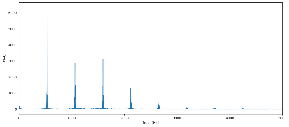
Let us now (pretend that we can actually) compute the DTFT of the trumpet signal, i.e.,
with \(s_n\) being the trumpet signal. (In practice, we are computing the DFT, but we will return to that later).
Example: An EEG Signal (eyes closed)#

Time-domain representation and frequency-domain representation (the spectrum) of anEEG signal with eyes closed. (a) The EEG signal is recorded at Oz and has a duration of 3 s and asampling rate of 160 Hz. By using bandpass filtering with difference cutoff frequencies, the signalcan be decomposed into five rhythms. (b) The spectrum of the EEG signal. After Zhang, Zhiguo. 2019. “Spectral and Time-Frequency Analysis,” in 89–116. doi:10.1007/978-981-13-9113-2_6. In “EEG Signal Processing and Feature Extraction”, edited by Li Hu and Zhiguo Zhang, 2019.
freqVector = np.arange(nData)*samplingFreq/nData # Hz
# we compute the DFT using an FFT algorithm
freqResponseClean = np.fft.fft(cleanTrumpetSignal)
ampSpectrumClean = np.abs(freqResponseClean)
plt.figure(figsize=(14,6))
plt.plot(freqVector,ampSpectrumClean,linewidth=2)
plt.xlim((0,5000)) # up to 5 KHz
plt.xlabel('freq. [Hz]'), plt.ylabel('$|X(\omega)|$');
Video example FFT (Live Code)#
We match the live script code from 16:27 to the end in the video exactly with python.
video = ipd.YouTubeVideo('QmgJmh2I3Fw', width=900, height=600)  # Accelerometer MATLAB Example
# Display the bigger video
display(video)
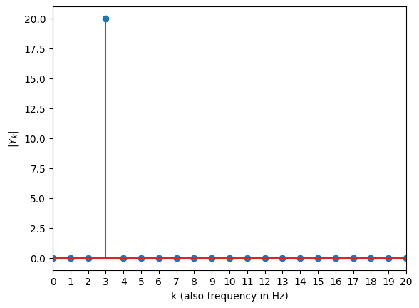
Sine Signal#
fs = 40
T = 1/fs
N = 40
# create time index for 1 seconds of a signal
t = np.arange(N)*T
# assign 3 Hz as frequency. TODO make it changable with a slider
xn = np.sin(2*np.pi*3*t)
One-sided FFT#
# One-sided FFT
Y = np.fft.fft(xn)
plt.figure
plt.stem(abs(Y))
# stem plot only up to half of Nyquist, make all integer ticks visible
plt.xticks(np.arange(0,N/2+1,1))
plt.xlim((0,N/2))
plt.xlabel('k (also frequency in Hz)'), plt.ylabel('$|Y_k|$')
plt.show()
# Note: we don't normalize to match the video, if we'd divide Y_3 to N/2 = 20, we would.
Example: a noisy trumpet signal#
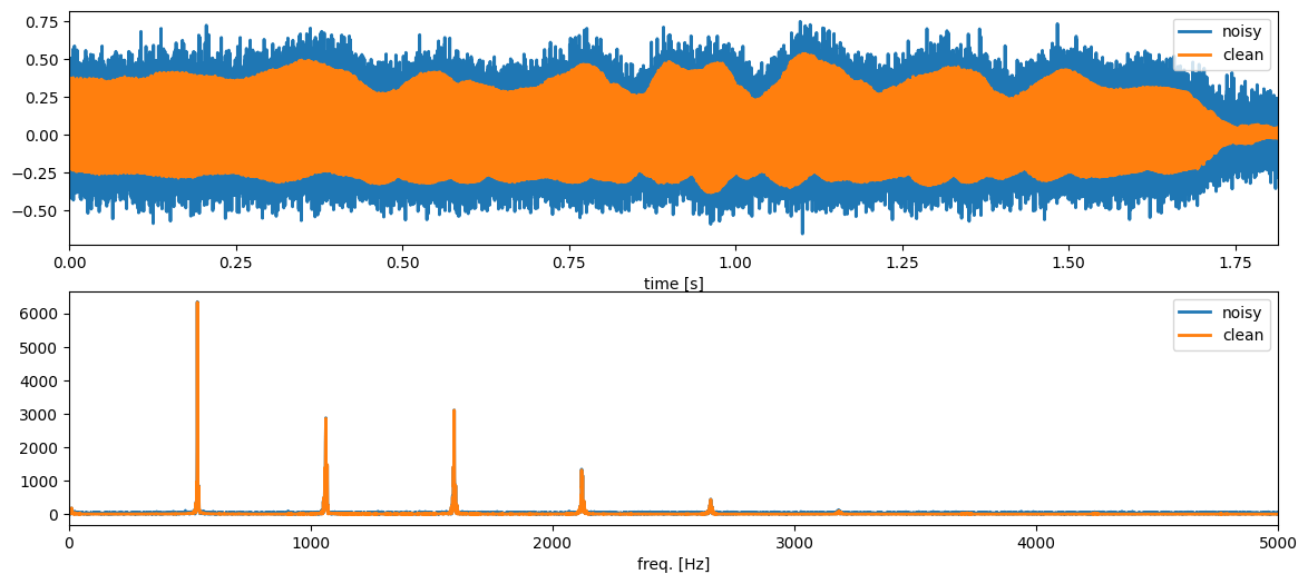
Let us now assume that we record a noisy trumpet signal. We can write this as $\( x_n = s_n + e_n \)$ where
\(x_n\) is the noisy trumpet signal
\(s_n\) is the clean (i.e., noise-free) trumpet signal
\(e_n\) is the noise
# add noise to the trumpet signal
noise = np.sqrt(0.01)*np.random.randn(nData) # generate so-called white Gaussian noise (WGN)
noisyTrumpetSignal = cleanTrumpetSignal + noise
freqResponseNoisy = np.fft.fft(noisyTrumpetSignal)
ampSpectrumNoisy = np.abs(freqResponseNoisy)
ipd.Audio(noisyTrumpetSignal, rate=samplingFreq)
In the frequency-domain, the noisy trumpet signal can be written as \begin{align} X(\omega) &= \sum_{n=-\infty}^{\infty} x_n \mathrm{e}^{-j\omega n} = \sum_{n=-\infty}^{\infty} (s_n+e_n) \mathrm{e}^{-j\omega n}\ &= \sum_{n=-\infty}^{\infty} s_n \mathrm{e}^{-j\omega n} + \sum_{n=-\infty}^{\infty} e_n \mathrm{e}^{-j\omega n}\ &= S(\omega)+E(\omega) \end{align} where
\(X(\omega)\) is the DTFT of the noisy trumpet signal
\(S(\omega)\) is the DTFT of the clean trumpet signal
\(E(\omega)\) is the DTFT of the noise
We see that the Fourier transform is additive. Thus, if we sum two signals in the time domain, we also sum them in the frequency domain. This is illustrated for the two signals \(x_n\) and \(y_n\) in the figure below.

plt.figure(figsize=(14,6))
plt.subplot(2,1,1)
plt.plot(timeVector,noisyTrumpetSignal,linewidth=2, label='noisy')
plt.plot(timeVector,cleanTrumpetSignal,linewidth=2, label='clean')
plt.xlim((timeVector[0],timeVector[-1])), plt.xlabel('time [s]'), plt.legend()
plt.subplot(2,1,2)
plt.plot(freqVector,ampSpectrumNoisy,linewidth=2, label='noisy')
plt.plot(freqVector,ampSpectrumClean,linewidth=2, label='clean')
plt.xlim((0,5000)), plt.xlabel('freq. [Hz]'), plt.legend();
Example task (SMC): removing noise from a trumpet signal#
Note that
the trumpet signal only has almost all of its energy concentrated in a few frequencies at (approximately) 530 Hz, 1060 Hz, 1590 Hz, 2120 Hz, 2650 Hz, etc. (These values have been estimated using a pitch estimator which we are going to discuss in lecture 12)
the noise is spread across all frequencies
we can remove a lot of noise by using a filter which will only allow the ‘trumpet frequencies’ to pass through
a feedback comb filter can be designed to do exactly that!

A feedback comb filter has the difference equation $\( y_n = x_n + a y_{N-D}\ . \)$
For a sampling frequency of \(f_\text{s} = 44,100\) Hz and a pitch of \(f_0 = 530 Hz\), the pitch period is $\( \frac{f_\text{s}}{f_0} = 83.08\ \text{samples} \)\( Since \)D\( has to be an integer, we will set \)D=83$ samples in the comb filter.

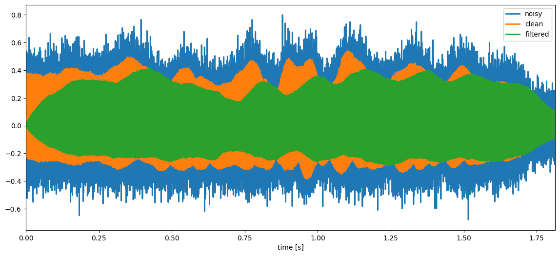
We will now remove the noise in the following way:
Filter the noisy trumpet signal \(x_n\) through the feedback comb filter given by $\( y_n = x_n + a y_{N-D} \)\( with \)D=83\( and \)a$ close (but not exceeding) 1.
The filter output \(y_n\) should now be much more similar to the clean trumpet signal \(s_n\) since the filter has removed a lot of noise.
# run a feedback comb filter to filter out the noise
def fbCombFiltering(noisySignal, delay, filterCoef):
    nData = np.size(noisySignal)
    filteredSignal = np.zeros(nData)
    for n in np.arange(nData):
        if n < delay:
            filteredSignal[n] = noisySignal[n]
        else:
            filteredSignal[n] = noisySignal[n]+filterCoef*filteredSignal[n-delay]
    return (1-filterCoef)*filteredSignal

pitchPeriod = 83 # samples (coarse estimate of the pitch period)
filterCoef = 0.98
filteredTrumpetSignal = fbCombFiltering(noisyTrumpetSignal, pitchPeriod, filterCoef)

plt.figure(figsize=(14,6))
plt.plot(timeVector,noisyTrumpetSignal,linewidth=2, label='noisy')
plt.plot(timeVector,cleanTrumpetSignal,linewidth=2, label='clean')
plt.plot(timeVector,filteredTrumpetSignal,linewidth=2, label='filtered')
plt.xlim((timeVector[0],timeVector[-1])), plt.xlabel('time [s]'), plt.legend()

ipd.Audio(filteredTrumpetSignal, rate=samplingFreq)
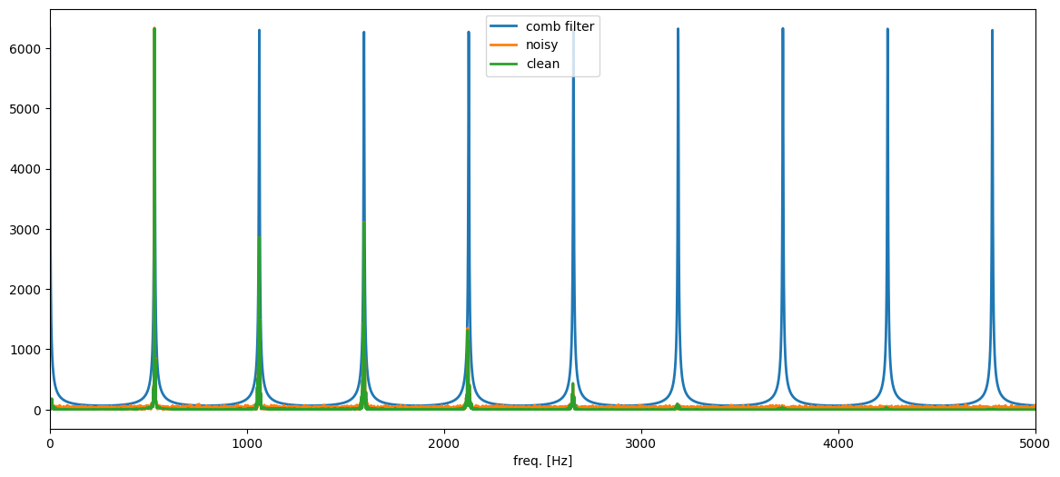
Example: transfer function and frequency response of the feedback comb filter#
In the last lecture, we saw that the transfer function of the feedback comb filter is $\( H(z) = \frac{1}{1-az^{-D}}\ . \)$
We can easily obtain the frequency response as the transfer function on the unit circle. That is, we set $\( z = \mathrm{e}^{j\omega} \)\( and obtain the **frequency response** of the comb filter to \)\( H(\omega) = \frac{1}{1-a\mathrm{e}^{-j\omega D}}\ . \)$
# compute the frequency response of the comb filter and normalise its maximum value
combFilterFreqResp = 1/(1-filterCoef*np.exp(-1j*(2*np.pi*freqVector/samplingFreq)*pitchPeriod))
combFilterFreqResp = (np.max(ampSpectrumClean)*(1-filterCoef))*combFilterFreqResp
plt.figure(figsize=(14,6))
plt.plot(freqVector,np.abs(combFilterFreqResp),linewidth=2, label='comb filter')
plt.plot(freqVector,ampSpectrumNoisy,linewidth=2, label='noisy')
plt.plot(freqVector,ampSpectrumClean,linewidth=2, label='clean')
plt.xlim((0,5000)), plt.xlabel('freq. [Hz]'), plt.legend();
Summary#
The discrete-time Fourier transform (DTFT) of a signal \(x_n\) is given by $\( X(\omega) = \sum_{n=-\infty}^{\infty} x_n \mathrm{e}^{-j\omega n}\ . \)\( You can think of the DTFT as a correlation between a signal and a *phasor* of frequency \)\omega$.
The inverse DTFT of a frequency response \(X(\omega)\) is given by $\( x_n = \frac{1}{2\pi}\int_{-\pi}^{\pi} X(\omega) \mathrm{e}^{j\omega n}d\omega\ . \)$ You can think of the inverse DTFT as writing the signal as a weighted sum of phasors.
Signals are often much easier to process and analyse in the frequency domain.
Active 5 minutes break#
Recall that an impulse is given by $\( \delta_n = \begin{cases} 1 & n=0\\ 0 & \text{otherwise} \end{cases}\ . \)$
Compute the frequency response of this impulse by computing the DTFT.
Assume that you pass the impulse through a filter (i.e., set \(x_n=\delta_n\)) with difference equation $\( y_n = x_n - x_{n-2}\ . \)\( 2. What is the impulse response \)h_n$ of this filter? 3. Compute the frequency response of the filter by computing the DTFT of the impulse response.
The DTFT of a signal/impulse response \(x_n\) is given by $\( X(\omega) = \sum_{n=-\infty}^{\infty} x_n \mathrm{e}^{-j\omega n}\ . \)$
Windowing#
In this part, you will learn
what a window is
why we need them
how windows change the frequency response of a signal
different types of windows
The DTFT of a signal response \(x_n\) is given by
Note that there are three practical problems with the DTFT
we will never observe a signal \(x_n\) from \(-\infty\) to \(\infty\)
the digital frequency \(\omega\) is a continuous parameter so we cannot store \(X(\omega)\) on a computer
the frequency content of most signals change as a function of time
We solve these problems using
windows to turn infinite signals into a finite number of non-zero samples (this block)
sample the DTFT on a uniform grid of frequencies (this is called the discrete Fourier transform (DFT)) (next block)
slide a window across a long signal to compute a short-time Fourier transform (STFT) (last block)
The rectangular window#
Let us first look at the rectangular window

We can think of the rectangular window \(w_n\) as a way of extracting the samples we see from an infinitely long signal \(x_n\), i.e.,

Example: DTFT of a window phasor#
Let us look at the phasor
\( x_n = \mathrm{e}^{j\omega_0 n} \)
which we observe for \(n=0,1,\ldots,N-1\).
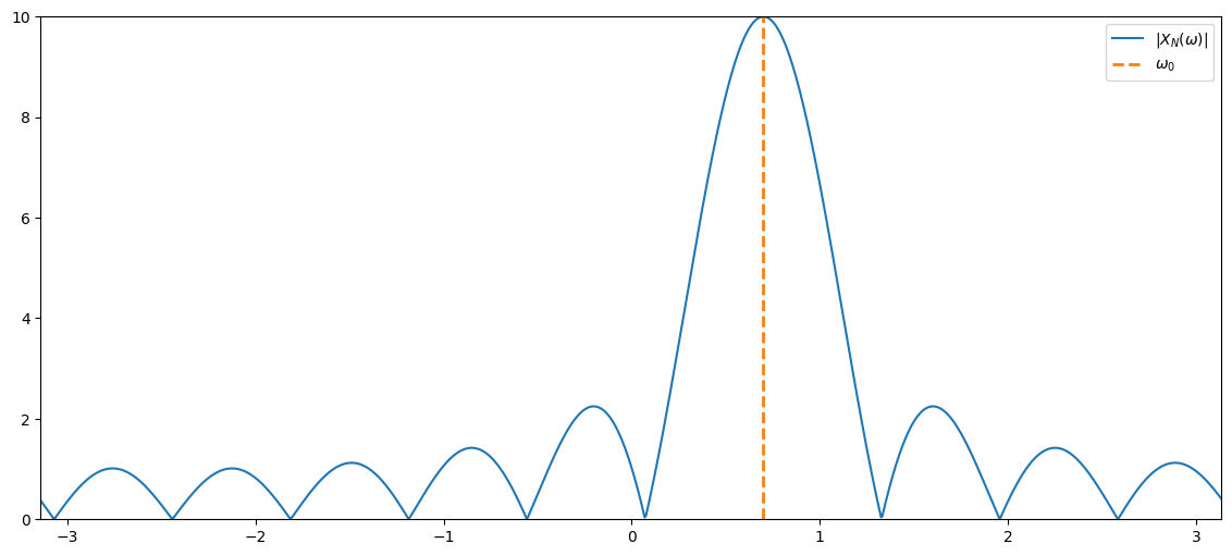
The DTFT of this windowed phasor is (note that subscript \(N\) in \(X_N(\omega)\) indicates the window length) \begin{align} X_N(\omega) &= \sum_{n=-\infty}^\infty (w_nx_n) \mathrm{e}^{-j\omega n} = \sum_{n=-\infty}^\infty (w_n\mathrm{e}^{j\omega_0 n}) \mathrm{e}^{-j\omega n}\ &= \sum_{n=0}^{N-1} \mathrm{e}^{j\omega_0 n} \mathrm{e}^{-j\omega n} = \sum_{n=0}^{N-1}\mathrm{e}^{-j(\omega-\omega_0) n}\ &= \frac{1-\mathrm{e}^{-j(\omega-\omega_0)N}}{1-\mathrm{e}^{-j(\omega-\omega_0)}} \end{align} where the last equality follows from the geometric series.
# %matplotlib inline
import numpy as np
import matplotlib.pyplot as plt

def computeDtftShiftedRectWindow(windowLength, freqShift):
    '''Compute the DTFT of a modulated rectangular window'''
    nFreqs = 100*windowLength
    freqGrid = 2*np.pi*np.arange(nFreqs)/nFreqs-np.pi
    complexNumber = np.exp(1j*(freqGrid-freqShift))
    numerator = 1-complexNumber**windowLength
    denominator = 1-complexNumber
    dtftShiftedRectWindow = np.zeros(nFreqs,dtype=complex)
    for ii in np.arange(nFreqs):
        if denominator[ii] == 0:
            # Using L'Hospital's rule, it can be shown that the DTFT is N when the dominator is 0
            dtftShiftedRectWindow[ii] = windowLength
        else:
            dtftShiftedRectWindow[ii] = numerator[ii]/denominator[ii]
    return dtftShiftedRectWindow, freqGrid
windowLength = 10
signalFreq = 0.7 # rad/sample
windowedDtft, freqGrid = computeDtftShiftedRectWindow(windowLength, signalFreq)

plt.figure(figsize=(14,6))
plt.plot(freqGrid,np.abs(windowedDtft), label='$|X_N(\omega)|$')
plt.plot(np.array([signalFreq,signalFreq]),np.array([0,windowLength]), '--', label='$\omega_0$')
plt.xlim((freqGrid[0], freqGrid[-1])), plt.ylim((0,windowLength)), plt.legend();
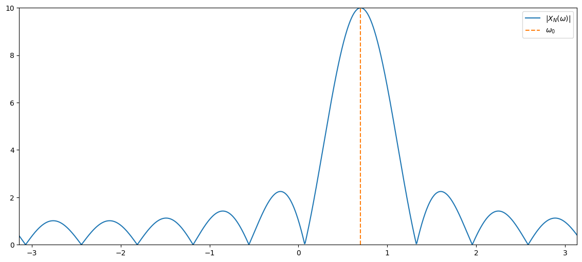
The windowed DTFT was $\( X_N(\omega) = \frac{1-\mathrm{e}^{-j(\omega-\omega_0)N}}{1-\mathrm{e}^{-j(\omega-\omega_0)}}\ . \)$
Note that
if we set \(w_0 = 0\), then \(x_n=1\) and we obtain the DTFT of only the window, i.e., $\( W_N(\omega) = \frac{1-\mathrm{e}^{-j\omega N}}{1-\mathrm{e}^{-j\omega}} \)$
rectWindowDtft,_ = computeDtftShiftedRectWindow(windowLength, 0)

plt.figure(figsize=(14,6))
plt.plot(freqGrid,np.abs(windowedDtft), label='$|X_N(\omega)|$')
plt.plot(np.array([signalFreq,signalFreq]),np.array([0,windowLength]), '--', label='$\omega_0$')
plt.plot(freqGrid,np.abs(rectWindowDtft), label='$|W_N(\omega)|$')
plt.xlim((freqGrid[0], freqGrid[-1])), plt.ylim((0,windowLength)), plt.legend();
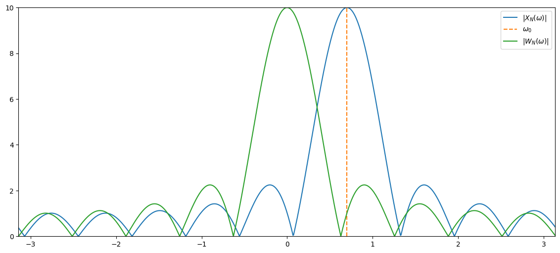
the DTFT \(X_N(\omega)\) of the windowed phasor is simply a frequency shifted version of \(W(\omega)\), i.e., $\( X_N(\omega) = W_N(\omega-\omega_0)\ . \)$ This is also called the modulation property of the DTFT.
if we let \(N\to\infty\), it can be shown that $\( \lim_{N\to\infty}X_N(\omega) =X(\omega) = \begin{cases} \infty & \omega = \omega_0\\ 0 & \text{otherwise} \end{cases}\ . \)\( Thus, the DTFT \)X(\omega)\( of a phasor of infinite duration has an infinite peak at \)\omega_0$ and is zero otherwise.
windowLength = 10
windowedDtftN, freqGridN = computeDtftShiftedRectWindow(windowLength, signalFreq)

plt.figure(figsize=(14,6))
plt.plot(freqGridN,np.abs(windowedDtftN), label='$|X_N(\omega)|$')
plt.plot(np.array([signalFreq,signalFreq]),np.array([0,windowLength]), '--', linewidth=2, label='$\omega_0$')
plt.xlim((freqGridN[0], freqGridN[-1])), plt.ylim((0,windowLength)), plt.legend();
Windowing and its influence of the DTFT#
Assume that we observe \(N\) samples of a signal \(x_n\) with DTFT \(X(\omega)\). How is the DTFT \(X_N(\omega)\) of the windowed signal related to \(X(\omega)\)? We know that the windowed DTFT and the inverse DTFT are given by \begin{align} X_N(\omega) &= \sum_{n=-\infty}^\infty w_nx_n\mathrm{e}^{-j\omega n} = \sum_{n=0}^{N-1} x_n\mathrm{e}^{-j\omega n}\ x_n &= \frac{1}{2\pi}\int_{-\pi}^\pi X(\tilde{\omega})\mathrm{e}^{j\tilde{\omega} n}d\tilde{\omega} \end{align} where we have added a \(\tilde{\cdot}\) on top of \(\omega\) in the last equation to indicate that it is an integration variable.
Inserting the last equation into the first results in $\( X_N(\omega) = \frac{1}{2\pi}\int_{-\pi}^\pi X(\tilde{\omega})\left[\sum_{n=0}^{N-1} \mathrm{e}^{j\tilde{\omega} n}\mathrm{e}^{-j\omega n}\right]d\tilde{\omega} = \frac{1}{2\pi}\int_{-\pi}^\pi X(\tilde{\omega})W(\omega-\tilde{\omega})d\tilde{\omega} \)\( which is a **convolution** between \)X(\omega)\( and the DTFT \)W(\omega)$ of the rectangular window.
video = ipd.YouTubeVideo('KuXjwB4LzSA')  # If you need a refresher, here is GREAT CONVOLUTION VIDE FROM 3BLUE1BROWN
# Display the video
display(video)
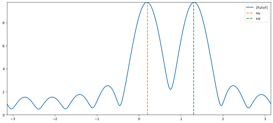
Note that applying a window is equivalent to low-pass filtering the DTFT \(X(\omega)\). This causes frequency smearing!

windowLength = 10
signalFreqA = 0.2 # rad/sample
signalFreqB = 1.3 # rad/sample
windowedDtftA, freqGrid = computeDtftShiftedRectWindow(windowLength, signalFreqA)
windowedDtftB, _ = computeDtftShiftedRectWindow(windowLength, signalFreqB)
windowedDtft = windowedDtftA+windowedDtftB

plt.figure(figsize=(14,6))
plt.plot(freqGrid,np.abs(windowedDtft), linewidth=2, label='$|X_N(\omega)|$')
plt.plot(np.array([signalFreqA,signalFreqA]),np.array([0,np.max(np.abs(windowedDtft))]), '--', linewidth=2, label='$\omega_A$')
plt.plot(np.array([signalFreqB,signalFreqB]),np.array([0,np.max(np.abs(windowedDtft))]), '--', linewidth=2, label='$\omega_B$')
plt.xlim((freqGridN[0], freqGridN[-1])), plt.ylim((0,np.max(np.abs(windowedDtft)))), plt.legend();
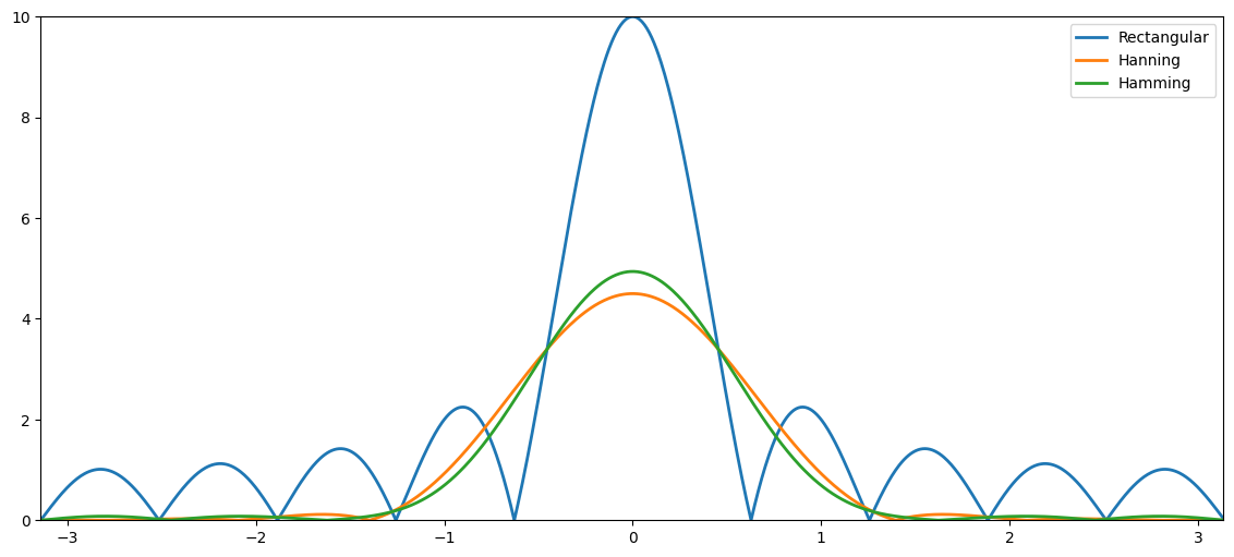
Bandwidth and sidelobes of windows#
Ideally, we would like a window with
narrow bandwidth to minimise frequency smearing
high sidelobe attenuation to minimise spectal leakage
Unfortunately, decreasing the bandwidth increases the sidelobes and vice versa for a fixed \(N\).

As no perfect window exists, many windows have been suggested. Note that
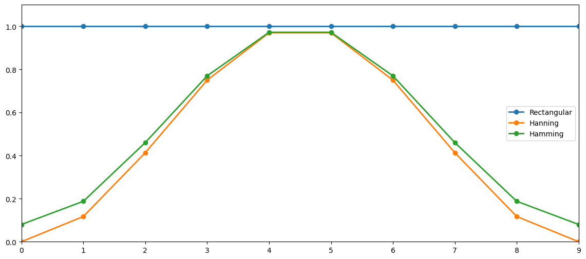
the windows have different trade-offs between bandwidth and sidelobe attenuation
examples of popular windows are rectangular, sine, Hamming, Hanning, Kaiser, and Gaussian. As an example, the hanning window is given by $\( w_n = \begin{cases} 0.5-0.5\cos(2\pi n/(N-1)) & n = 0, 1, \ldots, N-1\\ 0 & \text{otherwise}\ . \end{cases} \)$
the rectangular window has the smallest bandwidth and the lowest sidelobe attenuation
increasing the window length \(N\) decreases the bandwidth and increases the sidelobe attenuation.
# %matplotlib inline
import numpy as np
import matplotlib.pyplot as plt

windowLength = 10
samplingIndices = np.arange(windowLength)
rectWindow = np.ones(windowLength)
hanningWindow = np.hanning(windowLength)
hammingWindow = np.hamming(windowLength)

nDft = 1000
freqGrid = 2*np.pi*np.arange(nDft)/nDft-np.pi
dtftRectWindow = np.fft.fftshift(np.fft.fft(rectWindow,nDft))
dtftHanningWindow = np.fft.fftshift(np.fft.fft(hanningWindow,nDft))
dtftHammingWindow = np.fft.fftshift(np.fft.fft(hammingWindow,nDft))
plt.figure(figsize=(14,6))
plt.plot(samplingIndices,rectWindow,'o-',linewidth=2, label='Rectangular')
plt.plot(samplingIndices,hanningWindow,'o-', linewidth=2, label='Hanning')
plt.plot(samplingIndices,hammingWindow,'o-', linewidth=2, label='Hamming')
plt.xlim((samplingIndices[0],samplingIndices[-1])), plt.ylim((0,1.1)), plt.legend();
plt.figure(figsize=(14,6))
plt.plot(freqGrid,np.abs(dtftRectWindow), linewidth=2, label='Rectangular')
plt.plot(freqGrid,np.abs(dtftHanningWindow), linewidth=2, label='Hanning')
plt.plot(freqGrid,np.abs(dtftHammingWindow), linewidth=2, label='Hamming')
plt.xlim((freqGrid[0],freqGrid[-1])), plt.ylim((0,windowLength)),plt.legend();
Summary#
A window is used to extract a portion of a signal.
If we extract the \(N\) samples \(n=0,1,\ldots,N-1\), the windowed DTFT is $\( X_N(\omega) = \sum_{n=-\infty}^{\infty} w_n x_n \mathrm{e}^{-j\omega n} = \sum_{n=0}^{N-1} w_n x_n \mathrm{e}^{-j\omega n} \)$
Windowing a signal introduces frequency smearing and leakage, and these decrease as the window length increases
Many differenct windows exist and they trade-off the bandwidth for the sidelobe attenuation in different ways.
The discrete Fourier transform and Spectrograms#
In the next 20 minutes, you will learn
how the DFT is defined
how the DFT is related to the DTFT
what the short-time Fourier transform (STFT) is
what the spectrogram is
The discrete Fourier transform#
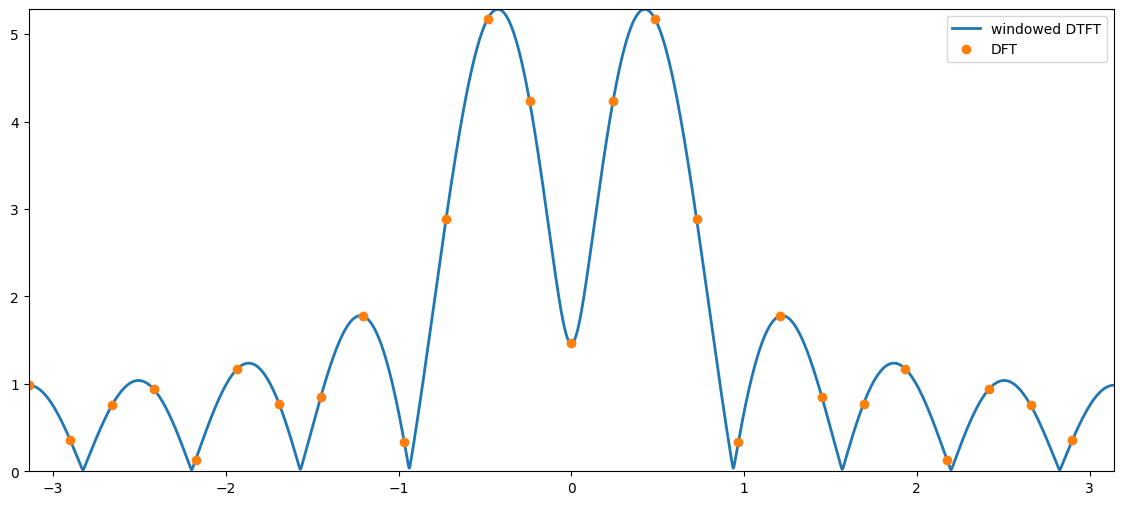
The discrete Fourier transform (DFT) is a sampled version of the windowed DTFT, i.e., $\( X_N(\omega_f) = \sum_{n=0}^{N-1} x_n \mathrm{e}^{-j\omega_f n} \)\( where the digital frequencies are evaluated on a \)F\(-point grid given by \)\( \omega_f = 2\pi f/F\qquad\text{for }f=0,1,\ldots,F-1 \)\( with \)F\geq N$.
Note that we have here assumed a rectangular window, but other windows can be used as well.
Often, the expression for \(\omega_f\) is inserted directly into the DFT definition and we obtain $\( X_N(\omega_f) = \sum_{n=0}^{N-1} x_n \mathrm{e}^{-j2\pi n f/F}\ . \)$
# %matplotlib inline
import numpy as np
import matplotlib.pyplot as plt

windowLength = 10
signalFreq = 0.3 # radians/sample
signal = np.cos(signalFreq*np.arange(windowLength))
nFreqsDtft = 2500
freqGridDtft = 2*np.pi*np.arange(nFreqsDtft)/nFreqsDtft-np.pi
windowedDtftSignal = np.fft.fftshift(np.fft.fft(signal,nFreqsDtft))
nFreqsDft = 26
freqGridDft = 2*np.pi*np.arange(nFreqsDft)/nFreqsDft-np.pi
dftSignal = np.fft.fftshift(np.fft.fft(signal,nFreqsDft))
plt.figure(figsize=(14,6))
plt.plot(freqGridDtft,np.abs(windowedDtftSignal), linewidth=2, label='windowed DTFT');
plt.plot(freqGridDft,np.abs(dftSignal), 'o', linewidth=2, label='DFT')
plt.xlim((freqGridDtft[0],freqGridDtft[-1])), plt.ylim((0,np.max(np.abs(windowedDtftSignal)))),plt.legend();
The inverse DFT#
Recall that the inverse DTFT is given by $\( x_n = \frac{1}{2\pi}\int_{-\pi}^{\pi} X(\omega) \mathrm{e}^{j\omega n}d\omega\ . \)$
The inverse DFT is given by $\( x_n = \frac{1}{F}\sum_{f=0}^{F-1} X(\omega_f) \mathrm{e}^{j\omega_f n} \)\( where \)\omega_f=2\pi f/F$.
The fast Fourier transform#
The fast Fourier transform (FFT) computes the DFT, but is a computationally efficient way.
Note that
computing the DFT directly from its definition costs in the order of \(F^2\) floating point (flops) operations (we write this as \(\mathcal{O}(F^2)\)).
computing the DFT using an FFT algorithm reduces the cost to just \(\mathcal{O}(F\log_2 F)\) flops
most FFT algorithms are working most efficiently when \(\log_2(F)\) is an integer
most FFT algorithms are slow (relatively speaking) if \(F\) is prime or has large prime factors (i.e., if you factorise \(F\) into a product of prime numbers and any of these are large, then most FFT algorithms will be slow)
entire books have been written on FFT algorithms, but the most important thing to remember is that they are all just different ways of compute the DFT as fast as possible!
The short-time Fourier transform (STFT)#
In most practical signals, the frequency content changes as a function of time.

Assume that we have a long signal \(x_n\) and a much shorter window \(w_n\) of length \(N\) which is zero everywhere, except for \(n=0,1,...,N-1\).
To analyse the signal, we slide it relative to the window. Mathematically, we can slide the signal by considering $\( x_{n+lL} \)$
for different \(l\) where
\(l\) is the frame index
\(L\) is the hop size.

If we combine this with a window of length \(N\), we obtain the STFT to $\( X_N(\omega_f, l) = \sum_{n=-\infty}^\infty w_n x_{n+lL} \mathrm{e}^{-j\omega_fn} = \sum_{n=0}^{N-1} (w_nx_{n+lL}) \mathrm{e}^{-j\omega_fn} \)$ which can be computed using the DFT.
Thus,
the STFT is simply a collection of DFTs computed at different positions of the signal
the samples we see through the window at a given position is called a frame or a segment and is indexed by the frame index \(l\)
unlike the DFT which only depends on the frequency index \(f\), the STFT also depends on the frame index \(l\)
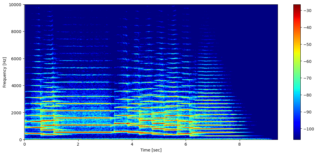
The spectrogram#
The spectrogram \(S_x(\omega_f,l)\) is the squared amplitude response of the STFT, i.e., $\( S_\text{x}(\omega_f,l) = |X_N(\omega_f, l)|^2\ . \)$
The spectrogram is used everywhere to visualise the frequency content as a function of time!
# %matplotlib inline
import numpy as np
import matplotlib.pyplot as plt
import scipy.signal as sig
import scipy.io.wavfile as wave
import IPython.display as ipd

def limitDynamicRange(spectrogram, maxRangeDb):
    minVal = np.max(spectrogram)*10**(-maxRangeDb/10)
    # set all values below minVal to minVal
    spectrogram[spectrogram < minVal] = minVal
    return spectrogram

# load a trumpet signal
samplingFreq, trumpetSignal = wave.read('data/trumpetFull.wav')
trumpetSignal = trumpetSignal/2**15 # normalise
ipd.Audio(trumpetSignal, rate=samplingFreq)
frameLength = int(np.round(0.05*samplingFreq)) # samples
hopSize = 0.75*frameLength # samples
nDft = 2**13
maxDynamicRange = 80 # dB
freqVector, timeVector, specgram = sig.spectrogram(trumpetSignal, \
    fs=samplingFreq, window=np.hanning(frameLength), nperseg=frameLength, noverlap=hopSize, nfft=nDft)
plt.figure(figsize=(14,6))
plt.pcolormesh(timeVector, freqVector, 10*np.log10(limitDynamicRange(specgram, maxDynamicRange)), cmap='jet')
plt.xlabel('Time [sec]'), plt.ylabel('Frequency [Hz]')
plt.colorbar(), plt.xlim((0,timeVector[-1])), plt.ylim((0,10000));
ipd.Audio(trumpetSignal, rate=samplingFreq)
Summary#
The discrete Fourier transform (DFT) is a sampled version of the windowed DTFT, i.e., $\( X_N(\omega_f) = \sum_{n=0}^{N-1} x_n \mathrm{e}^{-j\omega_f n} \)\( where \)\omega_f = 2\pi f/F\( for \)f=0,1,\ldots,F-1\( with \)F\geq N$.
The DFT can be computed efficiently using an FFT algorithm.
The short-time Fourier transform (STFT) is the DFT of different frames of the signal, i.e., $\( X_N(\omega_f, l) = \sum_{n=0}^{N-1} (w_nx_{n+lL}) \mathrm{e}^{-j\omega_fn} \)\( where \)l\( is the **frame index** and \)L$ the hop size.
The spectrogram is the squared amplitude response of the STFT.
Exercise SMC: Obtain the same STFT using librosa.#
# @title Solution (unhide if get stuck)
# calculate the STFT of the trumpet signal using librosa
import librosa

D = librosa.stft(trumpetSignal)  # STFT of y
S_db = librosa.amplitude_to_db(np.abs(D), ref=np.max)

plt.figure(figsize=(14,6))
# Change y axis up to 10kHz
plt.ylim(0,10000)
librosa.display.specshow(S_db, sr=samplingFreq, x_axis='time', y_axis='linear',cmap='jet')
plt.colorbar()
Exercise MED: Obtain a time-frewquency analysis of an EEG signal#
https://mne.tools/stable/auto_tutorials/intro/10_overview.html#time-frequency-analysis
# @title Solution (unhide if get stuck)
# calculate the STFT of the trumpet signal using librosa
!pip install mne --quiet
import numpy as np
import mne
sample_data_folder = mne.datasets.sample.data_path()
sample_data_raw_file = (
    sample_data_folder / "MEG" / "sample" / "sample_audvis_filt-0-40_raw.fif"
)
raw = mne.io.read_raw_fif(sample_data_raw_file)

# print(raw)
# print(raw.info)

raw.compute_psd(fmax=50).plot(picks="data", exclude="bads", amplitude=False)
raw.plot(duration=5, n_channels=30)
Epoching continuous data and time-frequency analysis#
The Raw object and the events array are the bare minimum needed to create an Epochs object, which we create with the Epochs class constructor. Here we’ll also specify some data quality constraints: we’ll reject any epoch where peak-to-peak signal amplitude is beyond reasonable limits for that channel type. This is done with a rejection dictionary; you may include or omit thresholds for any of the channel types present in your data. The values given here are reasonable for this particular dataset, but may need to be adapted for different hardware or recording conditions. For a more automated approach, consider using the autoreject package.
reject_criteria = dict(
    mag=4000e-15,  # 4000 fT
    grad=4000e-13,  # 4000 fT/cm
    eeg=150e-6,  # 150 µV
    eog=250e-6,
)  # 250 µV
events = mne.find_events(raw, stim_channel="STI 014")
event_dict = {
    "auditory/left": 1,
    "auditory/right": 2,
    "visual/left": 3,
    "visual/right": 4,
    "smiley": 5,
    "buttonpress": 32,
}

epochs = mne.Epochs(
    raw,
    events,
    event_id=event_dict,
    tmin=-0.2,
    tmax=0.5,
    reject=reject_criteria,
    preload=True,
)
319 events found on stim channel STI 014
Event IDs: [ 1  2  3  4  5 32]
Not setting metadata
319 matching events found
Setting baseline interval to [-0.19979521315838786, 0.0] s
Applying baseline correction (mode: mean)
Created an SSP operator (subspace dimension = 4)
4 projection items activated
Loading data for 319 events and 106 original time points ...
    Rejecting  epoch based on EEG : ['EEG 001', 'EEG 002', 'EEG 003', 'EEG 007']
    Rejecting  epoch based on EOG : ['EOG 061']
    Rejecting  epoch based on MAG : ['MEG 1711']
    Rejecting  epoch based on EOG : ['EOG 061']
    Rejecting  epoch based on EOG : ['EOG 061']
    Rejecting  epoch based on MAG : ['MEG 1711']
    Rejecting  epoch based on EEG : ['EEG 008']
    Rejecting  epoch based on EOG : ['EOG 061']
    Rejecting  epoch based on EOG : ['EOG 061']
    Rejecting  epoch based on EOG : ['EOG 061']
10 bad epochs dropped
conds_we_care_about = ["auditory/left", "auditory/right", "visual/left", "visual/right"]
epochs.equalize_event_counts(conds_we_care_about)  # this operates in-place
aud_epochs = epochs["auditory"]
vis_epochs = epochs["visual"]
del raw, epochs  # free up memory
Dropped 7 epochs: 121, 195, 258, 271, 273, 274, 275
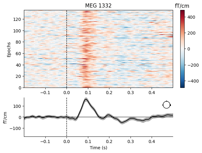
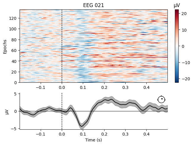
aud_epochs.plot_image(picks=["MEG 1332", "EEG 021"])
Not setting metadata
136 matching events found
No baseline correction applied
0 projection items activated
Not setting metadata
136 matching events found
No baseline correction applied
0 projection items activated
[<Figure size 640x480 with 4 Axes>, <Figure size 640x480 with 4 Axes>]
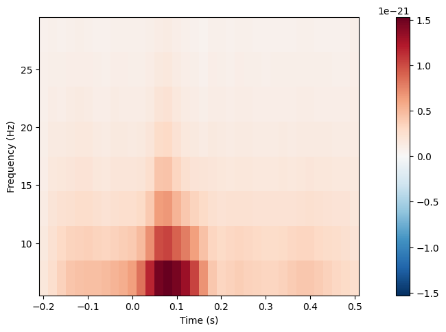
# Time-frequency
frequencies = np.arange(7, 30, 3)
power = aud_epochs.compute_tfr(
    "morlet", n_cycles=2, return_itc=False, freqs=frequencies, decim=3, average=True
)
power.plot(["MEG 1332"])
[Parallel(n_jobs=1)]: Done  17 tasks      | elapsed:    0.8s
[Parallel(n_jobs=1)]: Done  71 tasks      | elapsed:    2.6s
[Parallel(n_jobs=1)]: Done 161 tasks      | elapsed:    5.2s
[Parallel(n_jobs=1)]: Done 287 tasks      | elapsed:    8.8s
No baseline correction applied
[<Figure size 640x480 with 2 Axes>]