Lecture 3: The Fourier Transform - Signal Processing for Interactive Systems

Signal Processing for Interactive Systems

Aalborg University Copenhagen.

Last edited: 2026-02-26

The discrete-time Fourier transform¶

In this part, you will learn

why it is important to look at signals in the frequency domain
what the DTFT is
how you can visualise noise removal in the frequency domain

🔈 Understanding the DFT and the FFT (20 minutes): MATLAB Path is prefered. Content on MATLAB Online: You will be prompted to log in or create a MathWorks account. The project will be loaded, and you will see an app with several navigation options to get you started.

Example: analysing a trumpet signal Suppose that we record a trumpet signal $s_n$ for $n=0,1,2,\ldots,N-1$ .

try:
  import google.colab
  IN_COLAB = True
  !mkdir -p data
  !wget https://raw.githubusercontent.com/SMC-AAU-CPH/med4-ap-jupyter/main/lecture7_Fourer_Transfom/data/trumpet.wav -P data
  !wget https://raw.githubusercontent.com/SMC-AAU-CPH/med4-ap-jupyter/main/lecture7_Fourer_Transfom/data/trumpetFull.wav -P data
except:
  IN_COLAB = False


# %matplotlib inline
import numpy as np
import matplotlib.pyplot as plt
import scipy.io.wavfile as wave
import IPython.display as ipd
import librosa

# If needed you can load the trumpet full audio file, and crop the beginning for a single note as trumpet.wav
# audio_data, sampling_rate = librosa.load(librosa.ex('trumpet'))

# load a trumpet signal
samplingFreq, cleanTrumpetSignal = wave.read('data/trumpet.wav')
cleanTrumpetSignal = cleanTrumpetSignal/2**15 # normalise
ipd.Audio(cleanTrumpetSignal, rate=samplingFreq)

Loading...

nData = np.size(cleanTrumpetSignal)
timeVector = np.arange(nData)/samplingFreq # seconds
plt.figure(figsize=(14,6))
plt.plot(timeVector,cleanTrumpetSignal,linewidth=2)
plt.xlim((timeVector[0],timeVector[-1]))
plt.xlabel('time [s]'), plt.ylabel('$s_n$');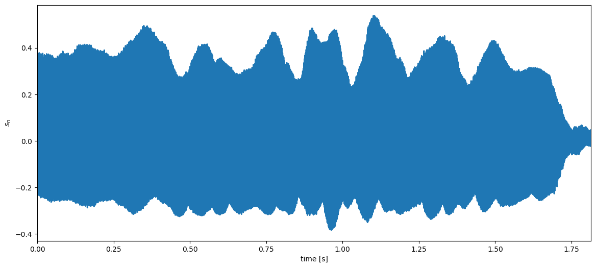

The discrete-time Fourier transform (DTFT)¶

Any colour can be written as a weighted combination of three atoms (red, green and blue colours).

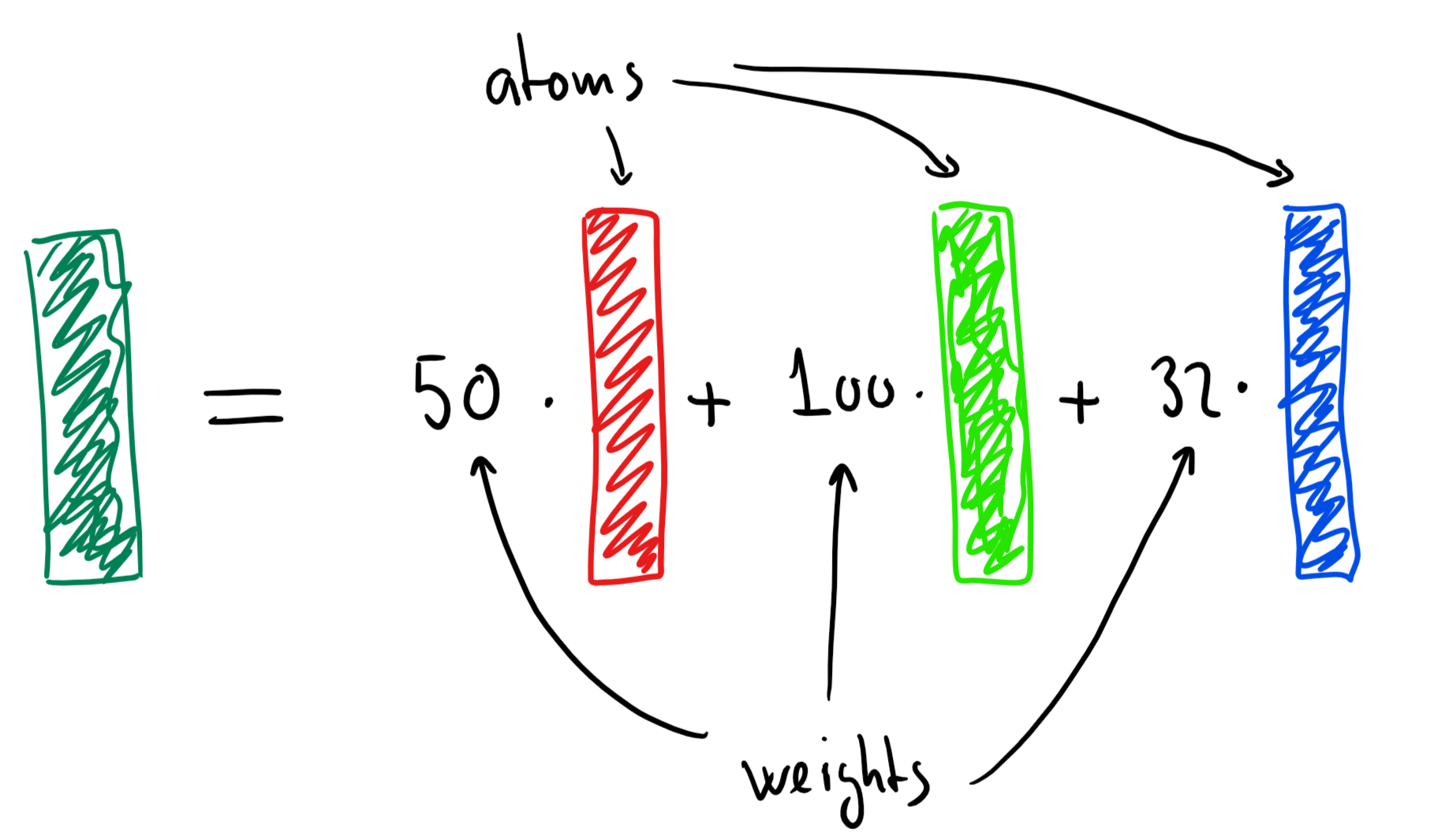
A signal (such as the trumpet signal) can be written as a weighted combination of phasors, i.e.,

s_n = \frac{1}{2\pi}\int_{-\pi}^{\pi} S(\omega) \mathrm{e}^{j\omega n}d\omega\ .

(1)

This is called the inverse discrete-time Fourier transform (inverse DTFT).

We can find the weights $S(\omega)$ by correlating our signal to the phasor $\mathrm{e}^{-j\omega n}$ , i.e.,

S(\omega) = \sum_{n=-\infty}^{\infty} s_n \mathrm{e}^{-j\omega n}\ .

(2)

This is called discrete-time Fourier transform (DTFT).

Note that

the DTFT is mostly of theoretical interest since we will never encounter infinitely long signals in practice
the practical version of the DTFT is called the discrete Fourier transform (DFT) (more on this later)

Example: analysing a trumpet signal¶

Let us now (pretend that we can actually) compute the DTFT of the trumpet signal, i.e.,

S(\omega) = \sum_{n=-\infty}^{\infty} s_n \mathrm{e}^{-j\omega n}\ ,

(3)

with $s_n$ being the trumpet signal. (In practice, we are computing the DFT, but we will return to that later).

Example: An EEG Signal (eyes closed)¶

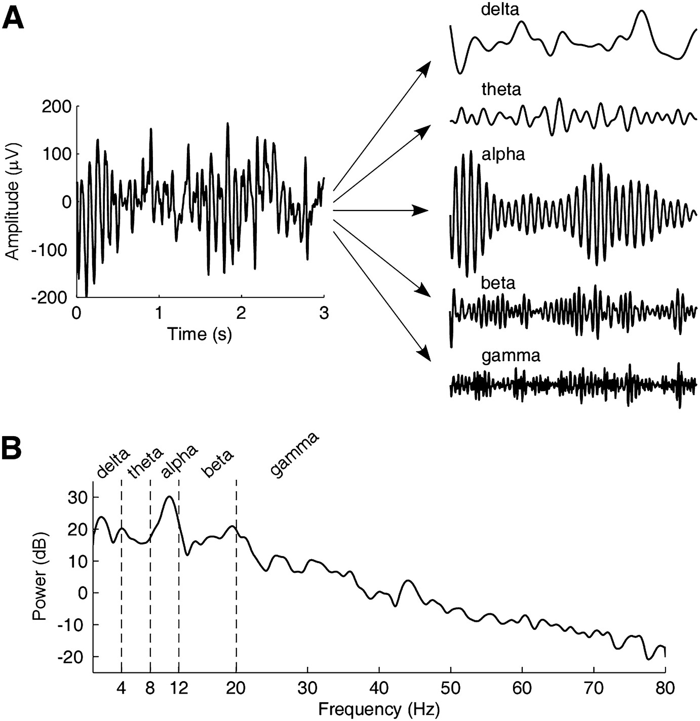
Time-domain representation and frequency-domain representation (the spectrum) of anEEG signal with eyes closed. (a) The EEG signal is recorded at Oz and has a duration of 3 s and asampling rate of 160 Hz. By using bandpass filtering with difference cutoff frequencies, the signalcan be decomposed into five rhythms. (b) The spectrum of the EEG signal. After Zhang, Zhiguo. 2019. “Spectral and Time-Frequency Analysis,” in 89–116. doi:10.1007/978-981-13-9113-2_6. In “EEG Signal Processing and Feature Extraction”, edited by Li Hu and Zhiguo Zhang, 2019.

freqVector = np.arange(nData)*samplingFreq/nData # Hz
# we compute the DFT using an FFT algorithm
freqResponseClean = np.fft.fft(cleanTrumpetSignal)
ampSpectrumClean = np.abs(freqResponseClean)
plt.figure(figsize=(14,6))
plt.plot(freqVector,ampSpectrumClean,linewidth=2)
plt.xlim((0,5000)) # up to 5 KHz
plt.xlabel('freq. [Hz]'), plt.ylabel('$|X(\omega)|$');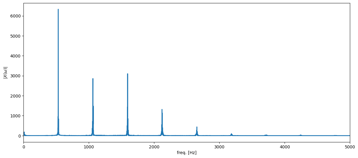

Sine Signal¶

fs = 40
T = 1/fs
N = 40
# create time index for 1 seconds of a signal
t = np.arange(N)*T
# assign 3 Hz as frequency. TODO make it changable with a slider
xn = np.sin(2*np.pi*3*t)

One-sided FFT¶

# One-sided FFT
Y = np.fft.fft(xn)
plt.figure
plt.stem(abs(Y))
# stem plot only up to half of Nyquist, make all integer ticks visible
plt.xticks(np.arange(0,N/2+1,1))
plt.xlim((0,N/2))
plt.xlabel('k (also frequency in Hz)'), plt.ylabel('$|Y_k|$')
plt.show()
# Note: we don't normalize to match the video, if we'd divide Y_3 to N/2 = 20, we would.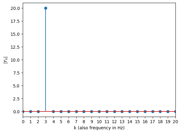

Example: a noisy trumpet signal (Anatomy of a classical-frequency domain DSP problem)¶

Let us now assume that we record a noisy trumpet signal. We can write this as

x_n = s_n + e_n

(4)

where

$x_n$ is the noisy trumpet signal
$s_n$ is the clean (i.e., noise-free) trumpet signal
$e_n$ is the noise

# add noise to the trumpet signal
noise = np.sqrt(0.01)*np.random.randn(nData) # generate so-called white Gaussian noise (WGN)
noisyTrumpetSignal = cleanTrumpetSignal + noise
freqResponseNoisy = np.fft.fft(noisyTrumpetSignal)
ampSpectrumNoisy = np.abs(freqResponseNoisy)
ipd.Audio(noisyTrumpetSignal, rate=samplingFreq)

Loading...

In the frequency-domain, the noisy trumpet signal can be written as

\begin{align} X(\omega) &= \sum_{n=-\infty}^{\infty} x_n \mathrm{e}^{-j\omega n} = \sum_{n=-\infty}^{\infty} (s_n+e_n) \mathrm{e}^{-j\omega n}\\ &= \sum_{n=-\infty}^{\infty} s_n \mathrm{e}^{-j\omega n} + \sum_{n=-\infty}^{\infty} e_n \mathrm{e}^{-j\omega n}\\ &= S(\omega)+E(\omega) \end{align}

(5)

where

$X(\omega)$ is the DTFT of the noisy trumpet signal
$S(\omega)$ is the DTFT of the clean trumpet signal
$E(\omega)$ is the DTFT of the noise

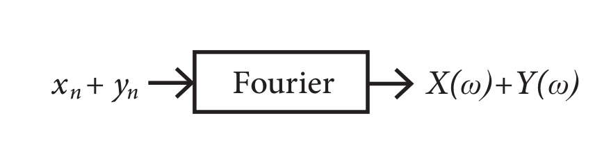
We see that the Fourier transform is additive. Thus, if we sum two signals in the time domain, we also sum them in the frequency domain. This is illustrated for the two signals $x_n$ and $y_n$ in the figure below.

plt.figure(figsize=(14,6))
plt.subplot(2,1,1)
plt.plot(timeVector,noisyTrumpetSignal,linewidth=2, label='noisy')
plt.plot(timeVector,cleanTrumpetSignal,linewidth=2, label='clean')
plt.xlim((timeVector[0],timeVector[-1])), plt.xlabel('time [s]'), plt.legend()
plt.subplot(2,1,2)
plt.plot(freqVector,ampSpectrumNoisy,linewidth=2, label='noisy')
plt.plot(freqVector,ampSpectrumClean,linewidth=2, label='clean')
plt.xlim((0,5000)), plt.xlabel('freq. [Hz]'), plt.legend();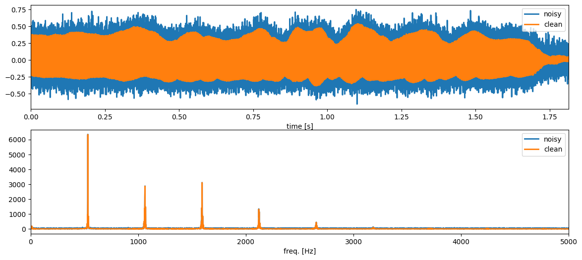

A typical SPIS Problem and towards a solution: removing noise from a trumpet signal¶

Note that

the trumpet signal only has almost all of its energy concentrated in a few frequencies at (approximately) 530 Hz, 1060 Hz, 1590 Hz, 2120 Hz, 2650 Hz, etc. (These values have been estimated using a pitch estimator which we are going to discuss in lecture 12)
the noise is spread across all frequencies
we can remove a lot of noise by processing the bands above a filter which will only allow the ‘trumpet frequencies’ to pass through.

Summary¶

The discrete-time Fourier transform (DTFT) of a signal $x_n$ is given by
$X(\omega) = \sum_{n=-\infty}^{\infty} x_n \mathrm{e}^{-j\omega n}\ .$
(6)
You can think of the DTFT as a correlation between a signal and a phasor of frequency $\omega$ .
The inverse DTFT of a frequency response $X(\omega)$ is given by
$x_n = \frac{1}{2\pi}\int_{-\pi}^{\pi} X(\omega) \mathrm{e}^{j\omega n}d\omega\ .$
(7)
You can think of the inverse DTFT as writing the signal as a weighted sum of phasors.
Signals are often much easier to process and analyse in the frequency domain.

The discrete Fourier transform¶

how the DFT is defined
how the DFT is related to the DTFT

The discrete Fourier transform¶

The discrete Fourier transform (DFT) is a sampled version of the windowed DTFT, i.e.,

X_N(\omega_f) = \sum_{n=0}^{N-1} x_n \mathrm{e}^{-j\omega_f n}

(8)

where the digital frequencies are evaluated on a $F$ -point grid given by

\omega_f = 2\pi f/F\qquad\text{for }f=0,1,\ldots,F-1

(9)

with $F\geq N$ .

💡Note that this can be interpreted as applying a rectangular window, a .

Often, the expression for $\omega_f$ is inserted directly into the DFT definition and we obtain

X_N(\omega_f) = \sum_{n=0}^{N-1} x_n \mathrm{e}^{-j2\pi n f/F}\ .

(10)

# %matplotlib inline
import numpy as np
import matplotlib.pyplot as plt

windowLength = 10
signalFreq = 0.3 # radians/sample
signal = np.cos(signalFreq*np.arange(windowLength))
nFreqsDtft = 2500
freqGridDtft = 2*np.pi*np.arange(nFreqsDtft)/nFreqsDtft-np.pi
windowedDtftSignal = np.fft.fftshift(np.fft.fft(signal,nFreqsDtft))
nFreqsDft = 26
freqGridDft = 2*np.pi*np.arange(nFreqsDft)/nFreqsDft-np.pi
dftSignal = np.fft.fftshift(np.fft.fft(signal,nFreqsDft))

plt.figure(figsize=(14,6))
plt.plot(freqGridDtft,np.abs(windowedDtftSignal), linewidth=2, label='windowed DTFT');
plt.plot(freqGridDft,np.abs(dftSignal), 'o', linewidth=2, label='DFT')
plt.xlim((freqGridDtft[0],freqGridDtft[-1])), plt.ylim((0,np.max(np.abs(windowedDtftSignal)))),plt.legend();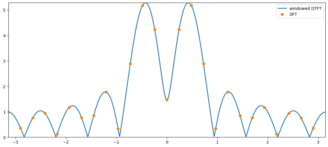

The inverse DFT¶

Recall that the inverse DTFT is given by

x_n = \frac{1}{2\pi}\int_{-\pi}^{\pi} X(\omega) \mathrm{e}^{j\omega n}d\omega\ .

(11)

The inverse DFT is given by

x_n = \frac{1}{F}\sum_{f=0}^{F-1} X(\omega_f) \mathrm{e}^{j\omega_f n}

(12)

where $\omega_f=2\pi f/F$ .

The fast Fourier transform¶

The fast Fourier transform (FFT) computes the DFT, but is a computationally efficient way.

Note that

computing the DFT directly from its definition costs in the order of $F^2$ floating point (flops) operations (we write this as $\mathcal{O}(F^2)$ ).
computing the DFT using an FFT algorithm reduces the cost to just $\mathcal{O}(F\log_2 F)$ flops
most FFT algorithms are working most efficiently when $\log_2(F)$ is an integer
most FFT algorithms are slow (relatively speaking) if $F$ is prime or has large prime factors (i.e., if you factorise $F$ into a product of prime numbers and any of these are large, then most FFT algorithms will be slow)
entire books have been written on FFT algorithms, but the most important thing to remember is that they are all just different ways of compute the DFT as fast as possible!

Summary¶

The discrete Fourier transform (DFT) is a sampled version of the windowed DTFT, i.e.,
$X_N(\omega_f) = \sum_{n=0}^{N-1} x_n \mathrm{e}^{-j\omega_f n}$
(13)
where $\omega_f = 2\pi f/F$ for $f=0,1,\ldots,F-1$ with $F\geq N$ .
The DFT can be computed efficiently using an FFT algorithm.